CHOOSE Function in Excel: Explained
In this article, you will learn how to use the CHOOSE formula in Excel.
What is the CHOOSE formula in Excel?
The CHOOSE formula in Excel is a function that allows you to select a value from a list of values based on a specified index number.
Why do you use the CHOOSE function in Excel?
The CHOOSE function in Excel is helpful because it allows you to select a value from a list of values based on a specified index number, which can be helpful in various situations. Some examples of when you might use the CHOOSE function include:
- Selecting an item from a list of things based on a user's selection: You can use the CHOOSE function to select an item from a list based on the index number that a user enters into a specific cell.
- Creating dynamic formulas: You can use the CHOOSE function to create dynamic functions that change based on a user's input. For example, you can use the CHOOSE function to select a different formula based on the value entered in a specific cell.
How to use the CHOOSE formula in Excel
The syntax of the formula is as follows:
"index_num" is the position of the value you want to select (e.g., 1 for the first value, 2 for the second value, etc.). This argument should be an integer between 1 and 254 or a cell reference containing a number within the range. If the number in this parameter is out of the range, the formula returns the #VALUE@ error value.
"value1, value2, ..." are the values from which you want to select. The “value1” is mandatory. This argument can accept numbers, dates, formulas, text, and cell references.
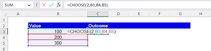
For example, if you have a list of values in cells B3:B5 and you want to select the value in cell B4, you would use the formula below:
How do you use the CHOOSE function for scenarios in Excel?
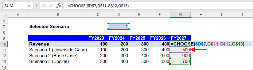
Assume you want to create three scenarios on your revenue forecast for the next five years - Upside, Base, and Downside cases for your financial analysis. You can insert the CHOOSE function in cells C10, D10, E10, F10, and G10. In each formula, the “value1”, “value2”, and “value3” should refer to the numbers of “Scenario 1”, “Scenario 2”, and “Scenario 3”, respectively, in the same column. In the example below, as the “index_num” is 1, the “value1” is returned in each cell containing the CHOOSE function. The following picture shows what the CHOOSE function in cell G10 looks like.
In the following example, we enter the CHOOSE functions in cells D20, E20, F20, and G20, in which the revenue growth changes depending on the selected scenario. Revenue is calculated based on the chosen growths. As the “index_num” is 3, each of the cells containing the CHOOSE formula returns 12% (“value3”). The function included in cell G20 is shown in the formula bar.

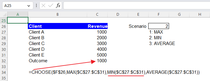
The last example shows the CHOOSE function containing other functions, specifically, MAX, MIN, and AVERAGE formulas. In the example, the formula returns the minimum value in cells C27:C31, which is 1000, because the “index_num” is 2 and the MIN function in “value2”, which finds the smallest number in a selected range, is applied to the range (C27:C31).
Analyze your live financial data in a snap in Google Sheets
Are you learning this formula to visualize financial data, build a financial model, or conduct financial analysis? In that case, LiveFlow may help you automate manual workflows, update numbers in real-time, and save time. You can access various financial templates on our website, from the simple Income Statement to Multi-Currency Consolidated Financial Statement. Are you interested in this product but are an Excel user? That’s not a problem at all. You can connect Google Sheets to Excel quickly.
To learn more about LiveFlow, book a demo.