
How to use INDEX & MATCH Function Together
Using the INDEX and MATCH functions together in Excel allows you to perform powerful and flexible lookups. Here's an example of how to use INDEX and MATCH together:
Sample Accounting Case Study
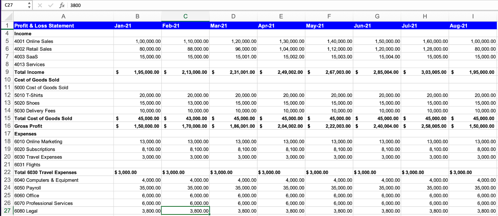
Assume you are an accountant and have Profit & loss data for the last 8 months in the format as shown below :
Suppose you wish to generate a summary dashboard that retrieves Profit and Loss data for a selected month chosen by the user from a drop-down menu. To accomplish this, you can utilize the INDEX function along with two MATCH functions by following the steps outlined below.
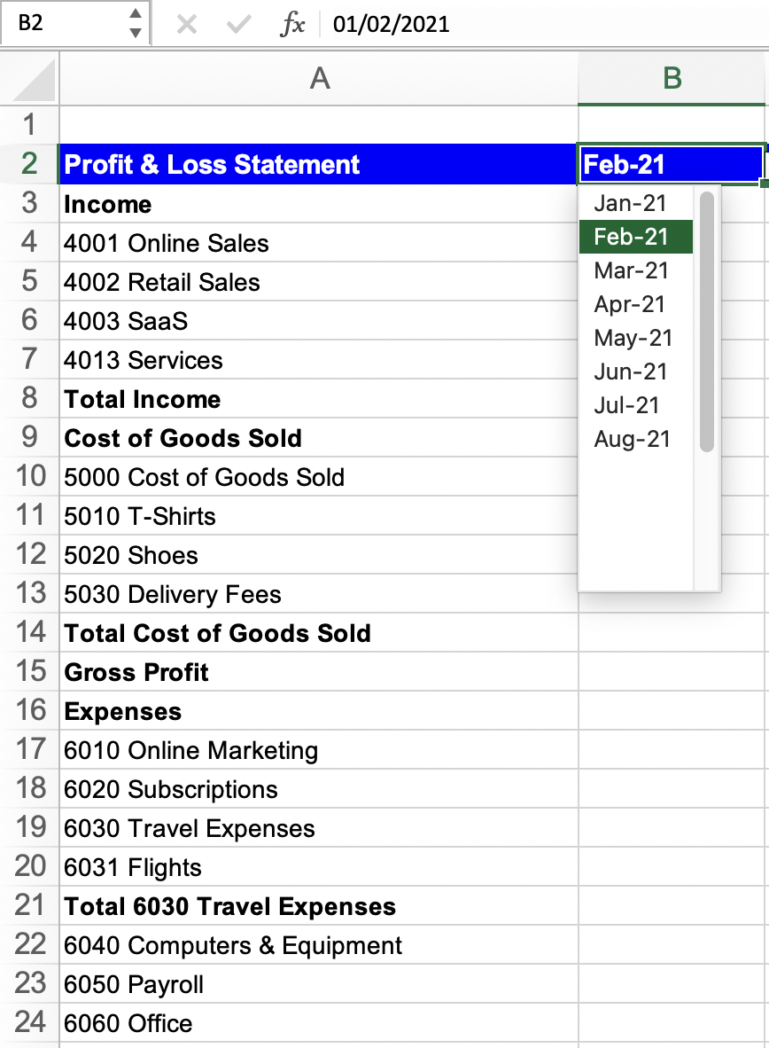
Step 1: Set up the summary tab with two columns where you can input the Profit and Loss Statement details and a drop-down for the month. Let's assume you have "Item Details" in column A and "Month drop-down" in cell B2.
Step 2: In the target cell where you want the Profit value to appear (let's say cell B4), use the following formula:
This formula combines the INDEX and MATCH functions, let us understand them separately
The INDEX function selects the value from the range $A$1:$I$40 in the Worksheet Profit & Loss (the entire Profit and Loss table in your workbook) based on the “row number” and “column number” provided by the MATCH functions.
The first MATCH function searches for a match between the Category Lookup value in A4 i.e. “4001 Online Sales” in the list of category names in column A of the Profit & Loss data set (A:A). The 0 at the end indicates an exact match. This function returns the row number of the matched category which in our case is 5. Do note we $A4 as we want to use the formula in subsequent rows.
The second MATCH function searches for a match between the Month Lookup value (B2) and the month names in the first row (1:1). The 0 at the end indicates an exact match and returns the column number of the matched month. Do note we use $B$2 &$1:$1 (with $ prefixes) to allow for the formula to be used in the subsequent rows.

Step 3: After entering the formula, press “Enter”. The formula will then retrieve the corresponding Profit value from the table for the month of Feb-21.
Step 4: Drag the formula in the subsequent rows to complete your Dashboard
Experiment by altering the month in the drop-down menu to observe the data refreshing in accordance with the user's selection.
By using the INDEX and MATCH functions together, you can dynamically retrieve data from a Profit and Loss dataset based on specific category and month combinations, allowing for flexible analysis and reporting.


