CHOOSEROWS Function in Excel: Explained

In this article, you will learn about the CHOOSEROWS Function and its uses in Excel.

‍

What is the CHOOSEROWS formula in Excel?

The CHOOSEROWS function in Excel is used to extract specific rows from an array or range. It returns an array of the specified rows in the order they are provided as arguments.

‍

Syntax of CHOOSEROWS function in Excel

The syntax of the Excel CHOOSEROWS function is as follows:

=CHOOSEROWS(array,row_num1,[row_num2],…)

The CHOOSEROWS function syntax has the following arguments:

array: This is the range or array of data from which you want to select rows.

row_num: Although these arguments can take a range as input,  you usually input a single integer, which specifies the row numbers to be returned from the array in each parameter. You can enter row numbers manually or use other Excel functions such as MATCH, INDEX, and SORT to generate the list of row numbers.

‍

Important note about the CHOOSEROWS function in Excel

Note that the CHOOSEROWS formula is only available in Excel for Microsoft 365 (Windows and Mac) and Excel for the web.

‍

How to Use CHOOSEROWS Function in Excel?

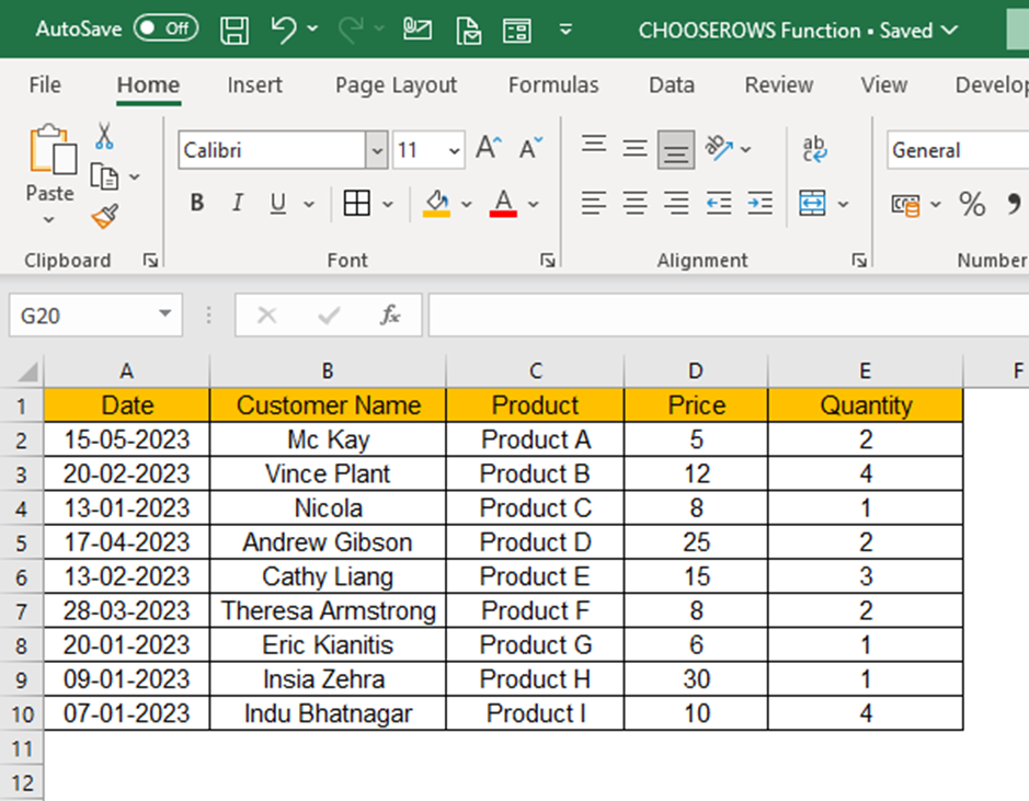
Understand the CHOOSEROWS function better with the help of an example case. The dataset below contains customer names and corresponding products purchased along with price, quantity, and date. Now the objective is to fetch the specific records from the database as per requirement.

‍

Mapping of the dataset with the syntax of the CHOOSEROWS function:

=CHOOSEROWS(array,row_num1,[row_num2],…)

array: In the example dataset, the array would be the range of cells from Cell A1:E10, which represents all cells in the table.

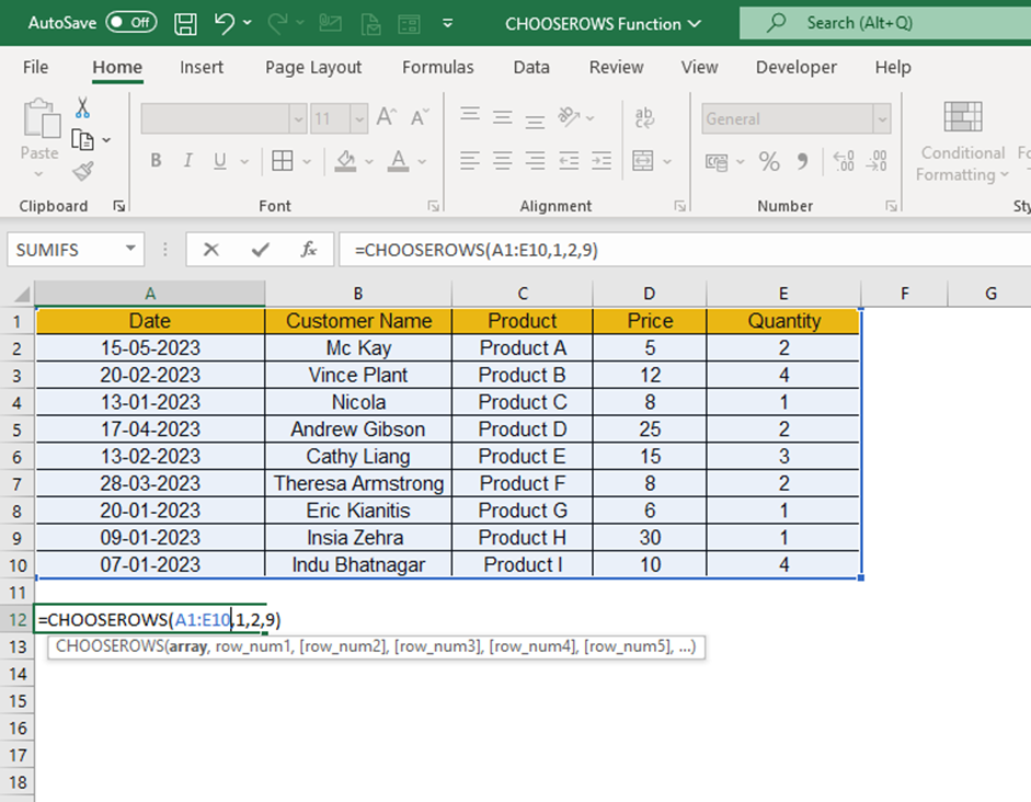
row_num: This shall be the row number that needs to be extracted from the dataset. For example, assume you pick up Row 1 containing the headers, Row 2 for “Mc Kay”, and Row 9 for “Insia Zehra”. Hence values input as row_num arguments will be 1,2,9.

Hence our complete function would look like this:

=CHOOSEROWS(A1:E10,1,2,9)

Now we need to apply this function in the corresponding cell A12 and press enter to generate the function result.

‍

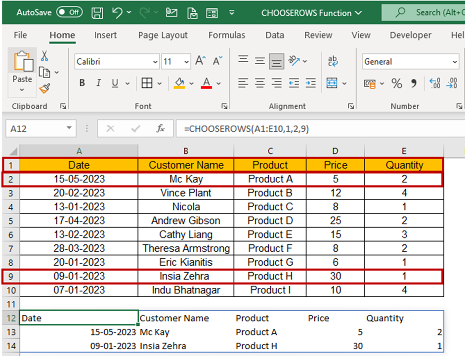
As you can observe, all the chosen rows appear instantly. This output is dynamic, so any change in source data would immediately reflect the same in this output.

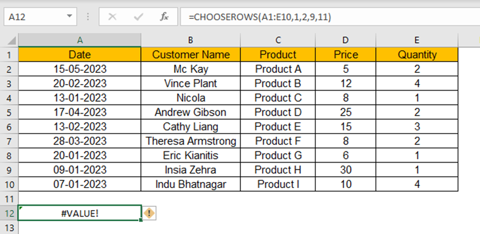
The formula gives you a #VALUE error if the absolute value of any of the row_num parameters is zero or exceeds the number of rows in the selected array.

Consider another scenario in the same sample dataset where we shall include another Row number 11 as part of the function. The updated function would look as below.

=CHOOSEROWS(A1:E10,1,2,9,11)

Now, if you update this function in Cell A12, it shall result in an error since one of the row numbers (11) exceeds the number of rows in the array (10). 

‍

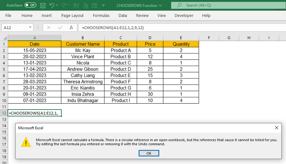
Consider another scenario in which one of your row_num parameters includes the row number of the cell where you are trying to place the CHOOSEROWS formula. In such a case, Excel would notify you of the circular reference error and restrict you from executing the function.

‍

When should you use the CHOOSEROWS Function in Excel? 

Here are some examples of when you might want to use the CHOOSEROWS function:

1. Retrieving the top or bottom rows of data: Suppose you have a large dataset with many rows and want to extract only the top or bottom rows based on a specific criterion, such as the highest or lowest values.
2. Randomly selecting rows from a dataset: Suppose you have a dataset with many rows, and you want to select a few rows for analysis or further processing randomly. You can use the CHOOSEROWS function and the RANDBETWEEN function to select rows from the dataset randomly.

‍

Errors potentially happen while using the CHOOSEROWS formula in Excel

If you encounter an error while using the CHOOSEROWS formula in Excel, it's most likely due to one of the following reasons.

1. Suppose you see a #VALUE! error, it means that the row_num argument is either zero or exceeds the total number of rows in the array.
2. If you see a #NAME? error, it means that the function's name is misspelled or the formula is not supported in your version of Excel. The CHOOSEROWS function is currently available only in Excel 365 and Excel for the web.
3. If you see a #SPILL! error, it means that there are not enough empty cells to display the results. To resolve this error, you can clear the cells blocking the results.