INDEX function in Excel: Explained

In this article, you will learn about the INDEX function in Excel.

‍

What does the INDEX function do?

The INDEX function in Excel is a powerful tool that allows you to retrieve the value from a specific position within an array or a range of cells. It is often used in combination with other functions to perform more complex calculations or data manipulations. Simply put, the INDEX function returns the value from the specified row and column within the array. It allows you to access individual elements of an array or extract specific data points from a range of cells.

‍

What are some uses of the INDEX function?

Following are a few examples of how the INDEX function can be used in Excel.

1. Retrieve a single value: You can use the INDEX function to fetch a specific value from a range or an array. By specifying the row number and column number, you can pinpoint the exact location of the desired value.
2. Create dynamic formulas: The INDEX function is often used in combination with other functions, such as MATCH or COUNTIF, to create dynamic formulas. For example, you can use INDEX and MATCH together to look up a value in a table based on certain criteria.
3. Extract rows or columns: By omitting the column_num parameter, the INDEX function can return an entire row of data based on the specified row number. Similarly, by omitting the row_num parameter, it can return an entire column.

This function provides flexibility in accessing data and is often combined with other functions to perform complex operations on your spreadsheet.

‍

How to use the INDEX function in Excel?

The syntax of the INDEX function is as follows:

=INDEX(array, row_num, [column_num])

array: This is the range or array of cells from which you want to retrieve the value.

row_num: This is the row number within the array where the value is located.

column_num: [Optional] This is the column number within the array where the value is located. If omitted, the INDEX function returns the entire row specified by row_num.

Here are the steps to use the INDEX function in Excel:

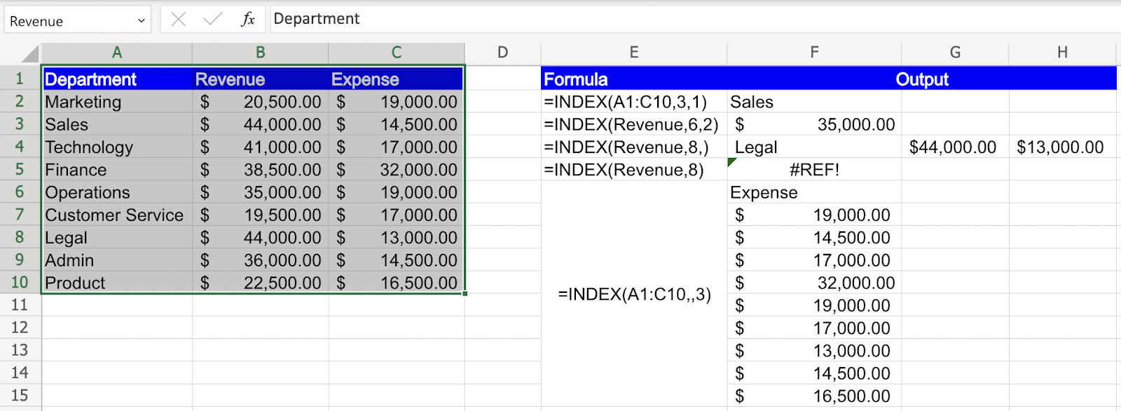
Step 1: Organize your data in a table or range in Excel or Identify the array or range of cells from which you want to retrieve data. This can be a single column, a single row, or a larger range in the below example this is A1:C10 or Named Range “Revenue”

Step 2: Choose the cell where you want to display the result of the INDEX function. In the selected cell, enter the INDEX function using the following syntax:

=INDEX(A1:C10,3,1)

Step 3: After entering the formula, press the Enter key to calculate the result. The INDEX function will retrieve the specified value from the array or range based on the provided row and column numbers. 

‍

By following these steps, you can effectively use the INDEX function in Excel to retrieve specific data points from your array or range of cells.

‍

‍