
TAKE Function in Excel: Explained
In this article, you will learn about the TAKE Function and its uses in Excel.
What is the TAKE formula in Excel?
The TAKE function in Excel is used to extract a specified number of contiguous rows or columns from the start or end of an array. Separate arguments for rows and columns are used to specify the desired number of rows and columns to return.
Syntax of the TAKE function in Excel
The syntax of the Excel TAKE function is as follows:
array: It is the array or range from which you want to extract rows or columns.
rows: It is the number of rows to extract. A positive value extracts rows from the start of the array, and a negative value extracts rows from the end of the array.
columns: It is the number of columns to extract. A positive value extracts columns from the start of the array, and a negative value extracts columns from the end of the array.
Note: The TAKE function is relatively new and only available in Excel for Microsoft 365 and the Web. If you are using an older version of Excel, you may be unable to use the TAKE function. One limitation is that the TAKE function can only extract contiguous rows or columns from an array. This means that you can only extract rows or columns next to each other. When either the number of rows or columns in Excel is set to 0, an empty array is indicated by the #CALC! error.
How to use the TAKE function in Excel?
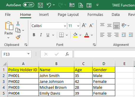
Understand how the TAKE function works in Excel by looking at particular examples. The below dataset contains information on policyholders, such as the policy ID, Name, Age, and Gender. Now the objective is to extract the first three rows from the array for showcasing in an Excel dashboard or a report.
Remember the general syntax of the TAKE formula as follows and think about how to replace the argument holders with your inputs as follows:
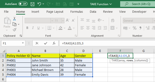
array: This will be the cell reference from A1:D5 to cover the entire dataset.
rows: This argument will be 3, since we need to extract the first three rows.
columns: We will ignore this argument as we would like to show all columns.
Hence our complete function would look as below:
Now we need to apply this function in cell F1 and press enter to generate the function result.
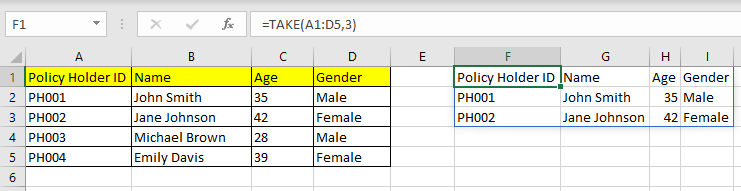
As you can see, the first three rows (from the left-hand side) are extracted from the original array and displayed in the defined position.
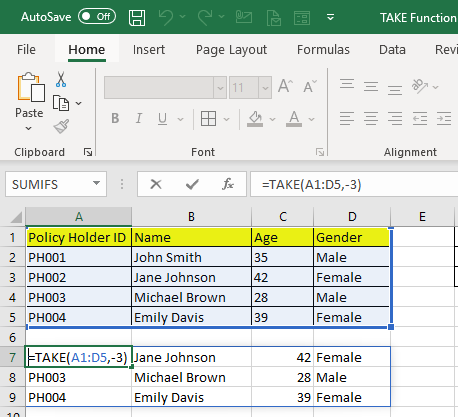
Next, consider a scenario where you need to extract the last three rows from the range, so we shall insert the following function:
Where -3 means to extract the three rows from the bottom of the array.
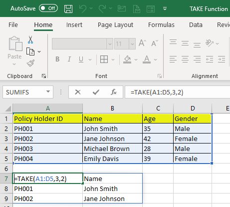
Further, look at another scenario where you pull the first three rows and first two columns from the initial data table, so we enter the following function:
Where 2 (column attribute) refers to extracting the first two columns of the source data table.
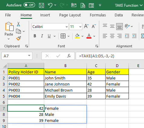
Assume a scenario where we extract the last three rows and last two columns from the range, so we insert the function as follows:
Where -3 (row attribute) means to pull out the last three rows from the array and -2 (column attribute) to quote the last two columns from the array.
When should you use the TAKE Function in Excel?
The TAKE function in Excel can be used in a variety of situations, but some of the most common uses include:
- Extracting a specific number of rows or columns from a large dataset: For example, you could use the TAKE function to extract the first 10 rows from a dataset of 1000 rows.
- Simplifying complex data structures: If you have a dataset that is organized in a complex way, you can use the TAKE function to extract the data into a simpler format. For example, you could use the TAKE function to extract all of the values from a column into a single row.
- Extracting specific data points: If you need to extract a specific data point from a dataset, you can use the TAKE function to do so. For example, you could use the TAKE function to extract the value in the first row and first column of a dataset.
- Creating new datasets: You can use the TAKE function to create new datasets from existing datasets. For example, you could use the TAKE function to create a new dataset that contains the first 10 rows of a larger dataset.
What is the difference between the TAKE and DROP functions in Excel?
The TAKE and DROP functions function in contrasting ways when returning a subset of an array. While the DROP function eliminates designated rows or columns from an array, the TAKE function retrieves specific rows or columns. The syntax of each function below would help you understand the difference.
=DROP(array,1) // the function shall remove the first row
=TAKE(array,1) // the function shall extract the first row


