GetPivotData function in Excel: Explained

In this article, you will learn how to use the GetPivotData formula in Excel.

‍

What does the GetPivotData formula do in Excel?

In Excel, the GETPIVOTDATA function is used to extract data from a pivot table. It retrieves data from a specific cell or cells in a pivot table by referencing the field names and items within the pivot table. 

‍

When you use the GETPIVOTDATA function, Excel generates a formula that references the pivot table and retrieves the corresponding data based on the specified field names and items. The function is particularly useful when you want to create dynamic reports or link specific cells outside the pivot table to retrieve summarized data.

How to use the GetPivotData function in Excel?

The syntax of the GetPivotData formula in Excel is as follows:

=GETPIVOTDATA(data_field, pivot_table, [field1, item1], [field2, item2], ...)

Here's a breakdown of the function's arguments:

data_field: This is the name of the value or data field that you want to retrieve from the pivot table. It is usually enclosed in double quotation marks.

pivot_table: This is a reference to a cell within the pivot table. You can simply click on a cell in the pivot table to automatically insert the reference.

[field1, item1], [field2, item2], ...: These are optional arguments that allow you to specify the field names and items to filter the data. You can include multiple field-item pairs to narrow down the data selection. These arguments follow the pattern [field, item].

‍

Note: When you copy or move a GETPIVOTDATA formula, Excel automatically adjusts the field and item references to match the new location, ensuring the formula continues to retrieve the correct data.

‍

Sample use case for the GetPivotData formula in Excel

Suppose you work for a retail company that sells various products across multiple regions. The company maintains a sales database that includes information about sales transactions, products, regions, and dates. You have been asked to analyze the sales data using a pivot table and extract specific information using GETPIVOTDATA.

‍

Step 1: Contains columns such as "Product," "Region," "Date," and "Sales Amount." 

Step 2: Create a Pivot Table based on the input data available using the following structure:

"Product" field into the "Rows" area, the "Region" field into the "Columns" area, and the "Sales Amount" field into the "Values" area. Ensure that the "Sales Amount" field is summarized as "Sum."

Step 3: You can now extract specific data Using GETPIVOTDATA for example you can retrieve the total sales amount for a specific product and region using: 

=GETPIVOTDATA("Sales Amount", PivotTable, "Product", "Product Name", "Region", "Region Name")

Replace "Product Name" and "Region Name" with the actual product and region names you want to analyze.

‍

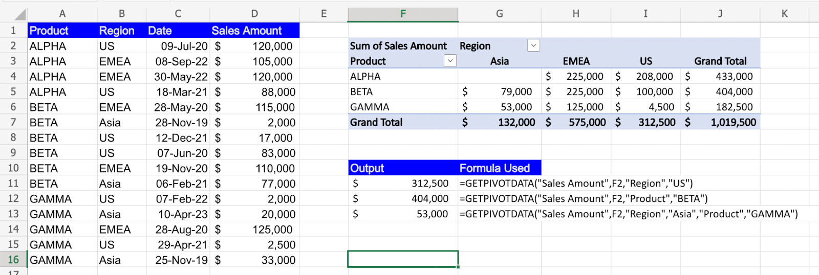
These examples demonstrate how you can use GETPIVOTDATA to retrieve specific data from the pivot table based on different criteria. You can further customize the formulas based on your specific analysis requirements.

‍

Note: Make sure to adjust the "PivotTable" reference in the GETPIVOTDATA formulas to match the actual cell reference of your pivot table.

‍