MATCH function in Excel: Explained

In this article, you will learn about the MATCH function in Excel.

‍

What does the MATCH function do?

The MATCH function in Excel is a useful tool that allows you to find the relative position of a specified value within a range or an array. It helps you locate the position of a value based on its position in a list or the criteria you specify. 

‍

What are some uses of the MATCH function?

Please see below for a few examples of how the MATCH function can be used in Excel. 

1. Finding the position of a value in a list: You can use the MATCH function to locate the position of a specific value within a range. It is helpful when you need to know the row number or the position of an item in a list or column.
2. Sorting or ranking data: The MATCH function can be used to sort or rank data based on certain criteria. By applying the MATCH function in an array formula, you can determine the position of values and use it to sort or rank the data accordingly.
3. Building dynamic formulas: The MATCH function is often used in combination with other functions such as INDEX to create dynamic formulas that adapt to changes in data. It allows you to find the position of a value dynamically and use it as a reference in various calculations or lookups.

‍

It provides flexibility in finding the position of a value within a range, enabling you to perform various data manipulations and calculations.

‍

How to use the MATCH function in Excel?

The syntax of the MATCH function is as follows:

=MATCH(lookup_value, lookup_array, [match_type])

lookup_value: This is the value you want to find within the lookup_array.

lookup_array: This is the range or array of cells in which you want to search for the lookup_value.

match_type: [Optional] This parameter specifies the type of match you want to perform. It can be set to 1, 0, or -1, representing different match types (0 or omitted: Exact match (default). 1: Finds the largest value less than or equal to the lookup_value. -1: Finds the smallest value greater than or equal to the lookup_value).

‍

The MATCH function returns the relative position of the lookup_value within the lookup_array. It can be used to determine the row number, column number, or position of a value within a range

To use the MATCH function in Excel, you can follow these steps:

‍

Step 1: Enter the data in two separate columns or ranges. One column or range will contain the values you want to search for, and the other column or range will be the reference range where you want to find those values.

Step 2: Select a cell for the formula, In the selected cell, type the formula to start the MATCH function. The syntax of the MATCH function is as follows:

=MATCH(lookup_value, lookup_array, [match_type])

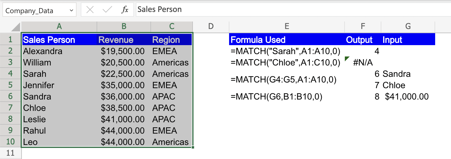
Step 3: Replace "lookup_value" in the MATCH function with either a specific value or a cell reference that contains the value you want to find for eg. “Sarah”. Similarly replace "lookup_array" in the MATCH function with the range of cells that you want to search for the lookup_value for example “A1:A10”. If desired, provide the "match_type" argument in the MATCH function to indicate the type of matching you want. 

Step 4: Press the Enter key to execute the formula. The result will be the position of the matched value within the lookup_array. If a match is found, it will display the relative position of the match. If no match is found or a larger lookup_array is provided, it will return an error value (#N/A).

‍

By following these steps, you can use the MATCH function in Excel to find the position of a value within a range or array.

‍

‍

‍