
MINIFS Function in Google Sheets: Explained
In this article, you will learn how to use the MINIFS formula in Google Sheets.
What does the MINIFS function do in Google Sheets?
The MINIFS function in Google Sheets is a function that returns the minimum value in a range that meets multiple criteria. The MINIFS formula is beneficial when searching a large amount of data for the lowest value that meets the requirements.
You can do the same search with the IF, MIN, and ARRAYFORMULA functions, but they tend to be complicated if you have multiple criteria, whereas the MINIFS formula allows you to build a clearer formula.
How to insert the MINIFS formula in Google Sheets
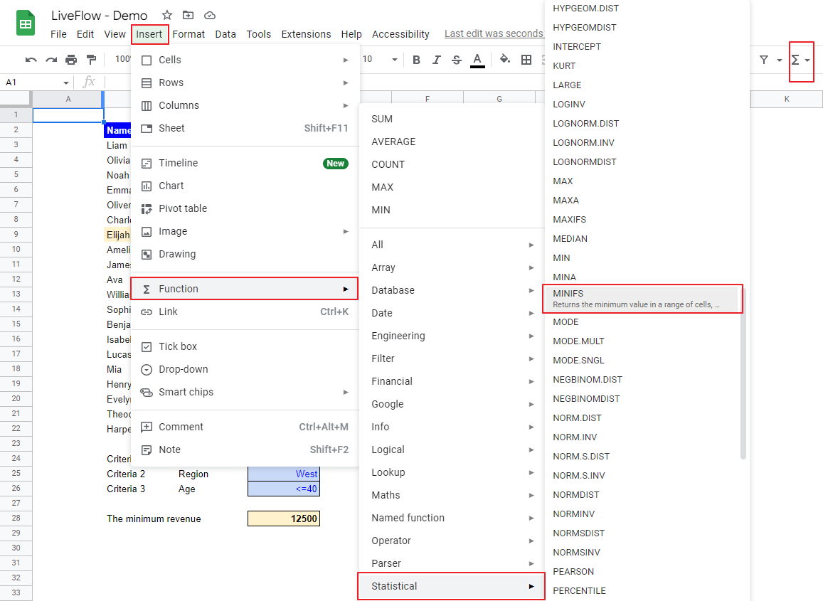
- Type “=MINIFS” or go to “Insert” → “Function” (or directly navigate to the “Functions” icon) → “Statistical” → “MINIFS”.
- Specify the range from which the formula finds the smallest value
- Input the range to which the function applies a criterion, and then the criterion
- Repeat the third step until you enter all criteria
- Press the “Enter” key.
In the next section, we will discuss how to use the MINIFS formula with examples.
How to use the MINIFS function in Google Sheets
The general syntax of the MINIFS formula is as follows:
range: This is the range that the function searched for the minimum value.
criteria_range1: This is the range to which the formula applies “criterion1”. The function checks whether each item in the range satisfies “criterion1”.
criterion1: This is a condition to filter the range, such as an amount of revenue or region of sales.
criteria_range2 [Optional]: Similar to “criteria_range1”, you need to specify the range to which the formula applies “criterion2”. You can select the same range with “criteria_range1” or a different one.
criterion2 [Optional]: If you need to input “criteria_range2”, you must identify the standard for the range.
Note 1: If necessary, you can add more than two criteria and their ranges
Note 2: The formula gives you zero if none of the conditions is met. Range and all of the criterion ranges need to be the same size. Otherwise, the MINIFS formula returns “#VALUE”.
Assume that you have a dataset containing information on your customers, such as customer ID, revenue amount, date, region, and age. You want to find the maximum revenue that meets the following conditions: sales recorded (i) after 12/1/2021, inclusive, (ii) in the “West” region, and (iii) by customers aged less than or equal to forty.
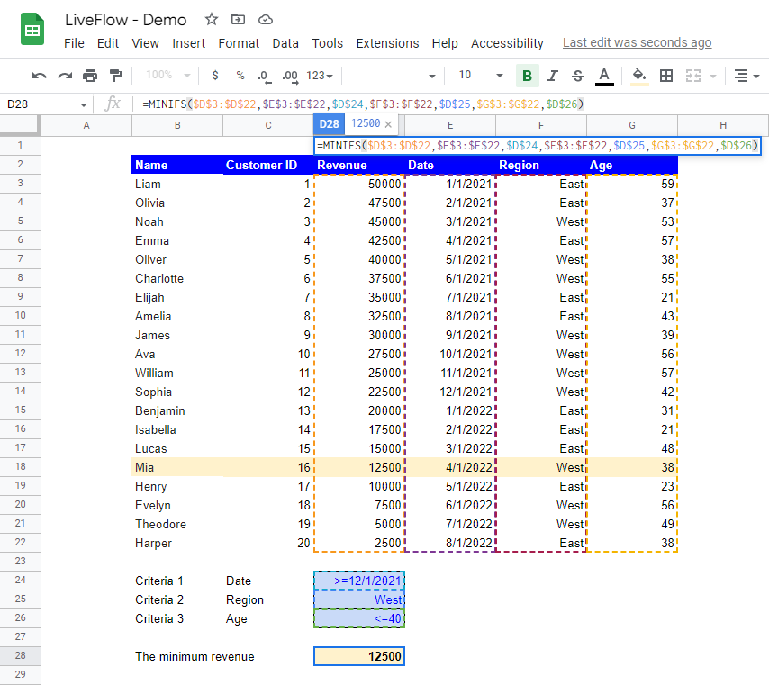
Look at the formula in detail. Note we fill two pairs of optional arguments for the second and third criteria (and the ranges to which they are applied).
range: $D$3:$D$22 (the Revenue column)
criteria_range1: $E$3:$E$22 (the Date column)
criterion1: $D$24 (Criteria 1)
criteria_range2: $F$3:$F$22 (the Region column)
criterion2: $D$25 (Criteria 2)
criteria_range3: $G$3:$G$22 (the Age column)
criterion3: $D$26 (Criteria 3)
As you can see, once you enter the Revenue range, what you need to do is to input a range for a criterion and the criterion and repeat the process until you include all three conditions. Then the formula automatically returns 12500, the minimum revenue meeting the abovementioned requirements.
When you use the MINIFS function, though you can input conditions manually in the formula, we highly recommend that you use cell references as we do because they allow you to see the requirements clearly and change them easily later, if necessary.
If you still want to use manual inputs for the formula, don’t enclose directly input arguments with quotation marks as you do for other functions.


