AVERAGEIFS Function in Google Sheets: Explained

In this article, you will learn how to use the AVERAGEIFS function in Google Sheets. The AVERAGEIFS function is helpful when you want to calculate the average of values under multiple standards. If you're going to calculate the average of values without any condition or with a condition, you should use the AVERAGE function or AVERAGEIF formula instead.

‍

How to use the AVERAGEIFS formula in Google Sheets

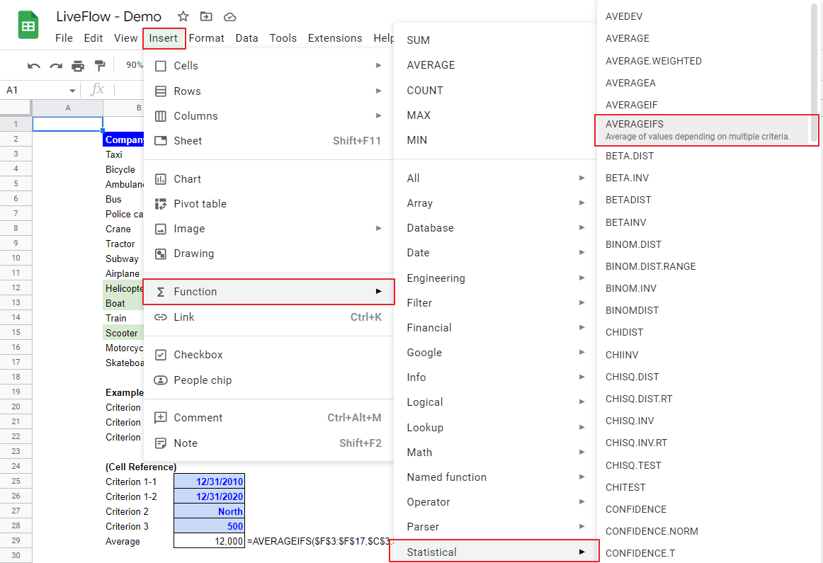
1. Type “=AVERAGEIFS” or navigate to “Insert” → “Function” → “Statistical” → “AVERAGEIFS”.
2. Select “average_range”. Next, choose “criteria_range1” for the first criterion and input “criterion1”.
3. Repeat inputting “criteria_range” and “criterion” until you incorporate all conditions in the formula.
4. Press the “Enter” key.

‍

The general syntax is as follows:

=AVERAGEIFS(average_range, criteria_range1, criterion1, [criteria_range2, …], [criterion2, …])

Average_range: This is the range containing the values (for numerator) based on which the formula calculates the average number. You can input a range you include as “criteria_range” in the “average_range”.

Criteria_range1: This is the range that the formula searches for the criterion. The formula counts the number of items that meet the first standard in the field (for the denominator)

Criterion1: This is a condition that an item incorporated in the average needs to meet. This value could be text, date, number, etc.

‍

In the end, the AVERAGEIFS function counts the number of items that meet all conditions incorporated in the formula and computes the average of their values.

‍

As mentioned at the beginning, this function is helpful when you want to compute the average figure depending on multiple criteria. With this function, you don’t need to calculate a total figure for a numerator and the number of items for a denominator separately to seek an average number.  Assume you are a finance manager and need to get an average revenue  of companies that meet the following conditions from the data set shown in the screenshot below.

‍

Condition 1: Establishment date is between 12/31/2010 and 12/31/2020 (including both beginning and end dates of the range)

Condition 2: Exists in “North” country

Condition 3: The number of employees is equal to or more than 500

‍

The formula in the screenshot above incorporates the following arguments.

Entire formula - cell reference version in cell C29 - is as follows:

=AVERAGEIFS($F$3:$F$17,$C$3:$C$17,$C$25,$C$3:$C$17,$C$26,$D$3:$D$17,$C$27,$E$3:$E$17,$C$28)

Average_range: $F$3:$F$17 - a column showing revenues

Criteria_range1: $C$3:$C$17 - a column showing establishment dates

Criterion1: $C$25 or “>=12/31/2010” (Manual Input)

Criteria_range2: $C$3:$C$17 - same as above

Criterion2: $C$26 or “<=12/31/2020” (Manual Input)

Criteria_range3: $D$3:$D$17 - a column showing countries

Criterion3: $C$27 or “North” (Manual Input)

Criteria_range4: $E$3:$E$17 - a column showing the number of employees

Criterion4: $C$28 or “>=500” (Manual Input)

‍

Criterion 1 and 2 correspond to Condition 1 (establishment date), Criterion 3 is tied with Condition 2 (country), and Criteiron 4 is for Condition 3 (employee number). Why do we have four criteria in the formula for the three conditions we assumed? That is because we broke down the first condition about the establishment dates into two bars in the AVERAGEIFS function.

‍

The formula calculates the average revenue of the companies highlighted in green after taking all requirements above into account.

‍

Key points are;

1. You should be clear about the criteria. Typing them down helps you understand and organize the requirements you want to include. Sometimes, you may need to break down a condition you come up with in the formula.
2. You can refer to a column more than once (as shown in the example - Column C) in the formula. 
3. For criteria inputs, cell reference is recommended because it allows you to change criteria flexibly by just typing new ones in cells referred, without opening a cell containing the AVERAGEIFS formula (to revise it). Also, in relation to the first point, clearly showing the criteria in cells helps you understand what conditions you have in the AVERAGEIFS formula.

‍

What is the difference between the AVERAGE and AVERAGEIFS?

The difference between AVERAGE and AVERAGEIFS functions is that the AVERAGE function simply calculates the average of values in a specified range, whereas the AVERAGEIFS function allows you to compute the average of values in a particular range depending on multiple conditions.

‍

Analyze your live financial data in a snap

Are you learning this function to visualize financial data, build a financial model, or conduct financial analysis? If so, LiveFlow may help you automate manual workflows and keep numbers updated in real-time. You can access more than fifty financial templates on our website, from the simple Income Statement to Multi-Currency Consolidated Financial Statement. You can also customize these templates as you want without breaking the automated data inflow.

To learn more about LiveFlow, book a demo.

‍

What are the other formulas related to mathematics and statistics

If you don’t get the solution you are looking for in this article, or you have further questions related to mathematics or statistics, you may find the answers in the following articles.

‍

Go to the following articles to learn basic formulas in Google Sheets.

How to Do Math in Google Sheets for Beginners

ADD Function in Google Sheets: Explained

MINUS Function in Google Sheets: Explained

DIVIDE Function in Google Sheets: Explained

MULTIPLY Function in Google Sheets: Explained

PRODUCT Function in Google Sheets: Explained

How to Use SUM Function in Google Sheets

How to Use SUMPRODUCT Formula in Google Sheets

How to Use MAX Function in Google Sheets

How to Use MIN Function in Google Sheets

How to Use MEDIAN Function in Google Sheets

How to Use AVERAGE Formula in Google Sheets

How to Use MODE Function in Google Sheets

MOD Function in Google Sheets: Explained

‍

Navigate to the pages below to learn how to sum, count, or average numbers with a condition or multiple conditions. 

How to Use SUMIF Function in Google Sheets - sum up the numbers that meet a criterion

SUMIFS Function in Google Sheets: Explained - sum up the numbers that meet multiple criteria

How to Use COUNTIF Function in Google Sheets - count the number of cells that meet a requirement

How to Use COUNTIFS function in Google Sheets - count the number of cells that meet multiple requirements

AVERAGEIF Function in Google Sheets: Explained - average the figures that meet a standard

AVERAGE.WEIGHTED Function in Google Sheets: Explained - use this formula to calculate the weighted average

MAXIFS Function in Google Sheets: Explained - seek for the maximum value that meets specific criteria

MINIFS Function in Google Sheets: Explained - seek for the minimum value that meets specific criteria

‍

Visit the following post if you are interested in learning how to count the number of specific cells.

COUNT Function in Google Sheets: Explained - count the number of cells containing numeric values (except for blank ones)

COUNTA Function in Google Sheets: Explained - count the number of cells incorporating all types of values containing text and date, except for blank ones

COUNTBLANK Function in Google Sheets: Explained - count the number of blank cells

COUNTUNIQUE Function in Google Sheets: Explained - count the number of unique cells

‍

You can learn about other Google Sheets formulas and tips that are not mentioned here on this page: LiveFlow‘s How to Guides