How to Use RANK Function in Google Sheets
In this article, you will learn how to utilize the RANK formula in Google. The Rank formula is beneficial when you want to rank each number in a range.
How to Use the RANK formula in Google Sheets
- Type “=RANK(” or go to “Insert” → “Function” → “Statistical” → “RANK”.
- Select a value whose rank is determined.
- Input a range containing all numbers you want to rank.
- Define how to rank numbers in ascending or descending order.

The generic syntax is as follows:
Value: This is a value whose rank is checked in the selected range.
Data: This is a data set including all figures you want to rank.
[is_ascending]: You can input 0 or 1. If you enter none of them, the formula assumes 0 is input. You can use “FALSE” and “TRUE” instead of 0 and 1, respectively
0 or “FALSE”: The function ranks the numbers in descending order. The greatest number is positioned in the first rank.
1 or “TRUE”: The formula ranks the values in ascending order. The lowest value is positioned in the first rank.
Assume you are in a corporate planning department and need to rank your clients in descending order according to the number of account receivables.

For instance, the arguments in the formula in cell D3 are as follows:
Value: C3
Data: $C$3:$C$12
[is_ascending]:FALSE
As it is efficient to copy the formula in cell D3 from D4 to D12 to evaluate all account receivables, we recommend you use the absolute reference for the “data” argument.
How do you rank from lowest to highest in sheets?
As described above, you can enter “1” or “TRUE” to rank figures in ascending order.
How do you find the top 5 in Google Sheets?
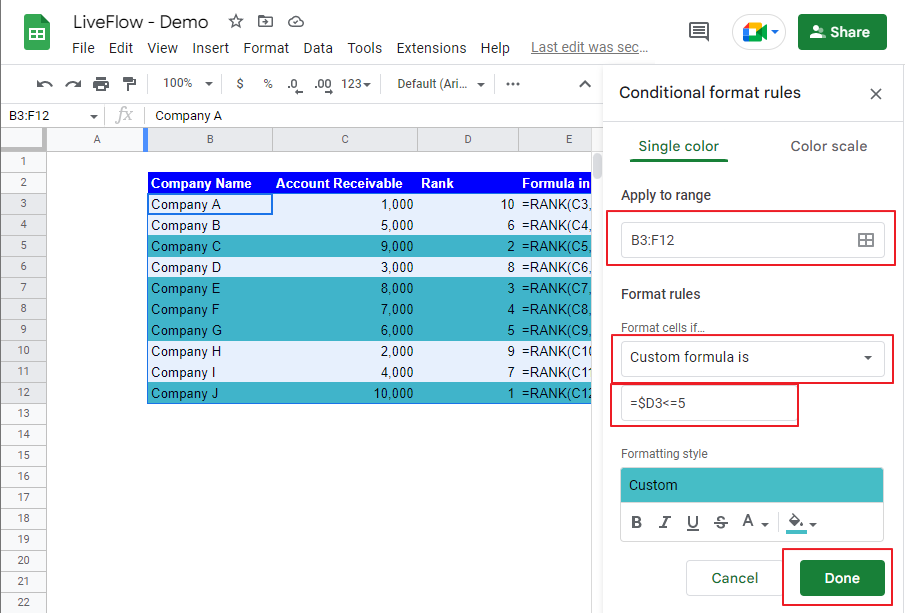
You can use Conditional Formatting to highlight the top 5 values in a range, assuming the largest value is the top. Assume you want to highlight the entire rows for the top 5 clients in the data set.
- Open the Conditional Formatting menu from the menu bar.
- Select the entire table.
- Choose “Custom formula is…” in Formula rules.
- Enter “=$D3<=5”*, which means cell format changes if the rank is equal to or lower than five (=top 5).
- Change “Formatting style”.
- Press “Done” at the bottom right.
*You must use the partial absolute reference because you want to use only the “Rank” Column (Column D) as a criterion for Conditional Formatting.