
AVERAGE.WEIGHTED Function in Google Sheets: Explained
In this article, you will learn how to use the AVERAGE.WEIGHTED formula in Google Sheets.
How does the AVERAGE.WEIGHTED formula work in Google Sheets?
The AVERAGE.WEIGHTED function in Google Sheets calculates the average of a data set, with the weighting of each value specified in a separate array of weights. The AVERAGE.WEIGHTED function can be helpful in situations where you want to give specific values more "importance" or "weight" in the average calculation.
For example, you could use this function if you are collecting data from multiple sources and you want to give more weight to data from sources that you consider more reliable. Another use case for this function is when you have a set of values that are not all equally important or relevant to your analysis.
For instance, you might have a list of customer ratings for a product, and you want to give more weight to ratings from customers who have made many purchases because you consider these ratings to be more representative of the overall satisfaction of your customer base.
How do you use the AVERAGE.WEIGHTED function in Google Sheets?
To use the AVERAGE.WEIGHTED function in Google Sheets, follow these steps:
- Select the cell where you want to display the result of the calculation.
- Type the following formula: “=AVERAGE.WEIGHTED”
- Enter a cell or a range to be averaged and a corresponding cell or range considered weight.
- If you want to include additional values and weights in the calculation, repeat step 3 for each additional value and its weight, if any.
- Press Enter to complete the formula and calculate the result.
The general syntax of the AVERAGE.WEIGHTED function is as follows:
values: These are the values from which you get the average value. You can input a specific value manually, reference a cell containing a value, or refer to a range containing values.
weights: These are the corresponding series of weights to be applied. Same as the “values”, you can fill this argument manually, or by cell reference. If you specify a range, the range should be the same size as the range referenced in “values”.
additional_values [Optional]: You can enter this value in the same way for “values”.
additional_weights [Optional]: You can enter this value similarly for “weights”.
Note: At least one of the weights should be positive. A negative weight is not accepted by the formula, though zero is allowed.
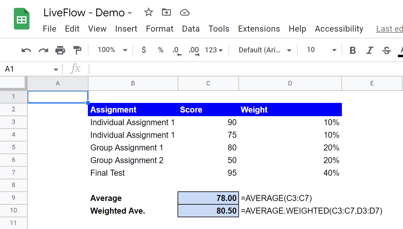
Suppose you have a list of assignments, their results, and corresponding weights in grading. You have assignment results in the range C3:C7, and corresponding weights in the range D3:D7. You can calculate the weighted average of these values with the following formula:
This will calculate the weighted average of the values in C3:C7, using the weights in D3:D7.
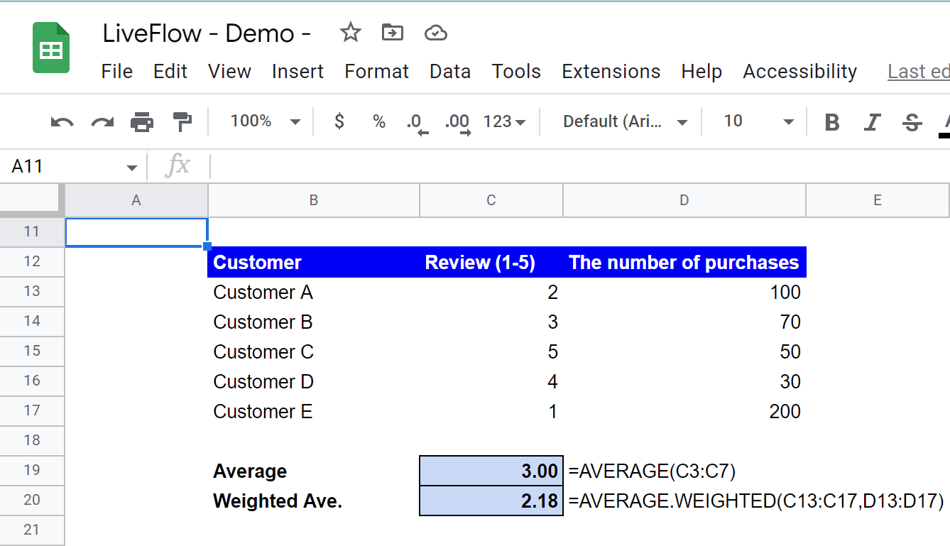
Look at another example. Assume you have customer data for an e-commerce website, such as customer name, each customer’s review on a specific product, and the number of purchases on the platform.
You have assignment results in the range C13:C17 and corresponding weights in the range D13:D17. You can calculate the weighted average of these values with the following formula:
This will calculate the weighted average of the values in C13:C17, using the weights in D13:D17.
In the two examples above, you can see the computed results by the AVERAGE.WEIGHTED formula are different from the values returned by the AVERAGE formula.


