COUNTIFS Function in Excel: Explained
In this article, you will learn how to use the COUNTIFS formula in Excel.
How does the COUNTIFS formula work in Excel?
The COUNTIFS formula in Excel allows you to count the number of cells in a range that meet multiple criteria.
When do you use the COUNTIFS function in Excel?
The COUNTIFS function in Excel is typically used when you need to count the number of cells in one or more ranges that meet multiple criteria. For example, you could use the COUNTIFS formula to count the sales of a specific product in a particular region or the number of students who received a certain grade in a specific class. This function is often used in data analysis and reporting and can help you quickly and easily identify trends and patterns in your data.
How to use the COUNTIFS formula in Excel
The general syntax for the formula is as follows:
The first range and criteria are required, but you can add additional ranges and criteria as needed.
"criteria_range1" is the range of cells that you want to evaluate using the "criteria1" condition.
"criteria1" is the condition that the cells in "criteria_range1" must meet to be included in the count.
"criteria_range2", "criteria2", etc. are optional arguments, where you can include other ranges and conditions that cells must meet to be included in the count.
Note 1: The formula returns the number of cells that meet all specified conditions.
Note 2: All “criteria_range” arguments must be the same size and shape.
Note 3: When you enter non-numeric criteria manually in the formula, remember that you enclose each text with double quotes.
Note 4: The COUNTIFS formula is not case-sensitive.
In the next section, you can see examples of the COUNTIFS function with multiple conditions, such as numeric value and text.
How to use the COUNTIFS function with multiple criteria in Excel
Before looking at some examples, learn basic operators and wildcards quickly.
If you can add a condition to a specific number of N, you can use the following logic operators.
>N: Greater than N
>=N: Greater than or equal to N
<N: Less than N
<=N: Less than or equal to N
=N: Equal to N
<>N: Not equal to N
Wildcards include three signs: an asterisk, a question mark, and a tilde, each of which has a different function.
”*” (Asterisk): Any character (e.g., “A*”: Any characters starting with A / “*B*”: Any characters containing B)
”?” (Question mark): The number of character(s) corresponds to the number of question mark(s). (e.g., ”????”: Any four characters)
”~” (Tilde): This negates the effect of the other wildcards next to the right and makes them work as literal marks without any function as wildcards. (e.g., ”*~?~?*”: Any characters containing two question marks)
Number and Text
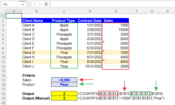
Assume you have the dataset in the following picture and want to compute the number of clients who recorded sales over 5000 and bought Pear. You can use the following COUNTIFS formula:
criteria_range1: $E$3:$E$12 (Sales column)
criteria1: $C$15
criteria_range2: $C$3:$C$12 (Product Type column)
criteria2: $C$16
Although we recommend that you use cell references to input conditions as they give you more visibility and clarity of the criteria applied, if you can insert the criteria manually, you can create the formula below for this case.
Text and Date
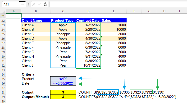
Next, imagine you have the same dataset and want to calculate the number of clients who purchased products whose names do not start with P on or before 6/30/2022. The formula should be as follows:
criteria_range1: $C$23:$C$32 (Product Type column)
criteria1: $C$35
criteria_range2: $D$23:$D$32 (Contract Date column)
criteria2: $C$36
The following formula includes input criteria manually.
Date and Number
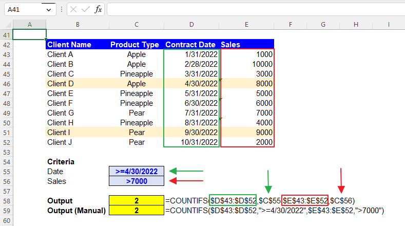
Lastly, assume that you have the same dataset and want to calculate the number of clients who recorded more than 7000 sales on or after 4/30/2022. You can use the formula below.
criteria_range1: $D$43:$D$52 (Contract Date column)
criteria1: $C$55
criteria_range2: $E$43:$E$52 (Sales column)
criteria2: $C$56
If you want to generate the COUNTIFS formula with manually input conditions, use the formula below.
Why do you use cell references in the COUNTIFS formula in Excel?
As you have seen, you can input the “criteria” argument(s) manually. However, we recommend the cell reference approach (instead of manual inputs) because it gives you more visibility and clarity about the condition as the requirement can be seen in a cell and allows you to change the standard more quickly. You don’t need to put your cursor on the cell containing the formula or open the cell by hitting the F2 button to see in detail or revise the function. Note that you don’t need to enclose it with quotation marks when you put a criterion in a cell.
What is the difference between the COUNTIFS and COUNTIF functions in Excel?
The COUNTIF and COUNTIFS functions in Excel are used to count the number of cells in a range. However, there is a key difference between the two functions. The COUNTIF function only allows you to count the number of cells that meet a single criterion, whereas the COUNTIFS function allows you to count the number of cells that meet more than one condition. Therefore, if you have multiple conditions you want to apply to a dataset, you should use the COUNTIFS function.
Analyze your live financial data in a snap in Google Sheets
Are you learning this formula to visualize financial data, build a financial model, or conduct financial analysis? In that case, LiveFlow may help you automate manual workflows, update numbers in real-time, and save time. You can access various financial templates on our website, from the simple Income Statement to Multi-Currency Consolidated Financial Statement. Are you interested in this product but are an Excel user? That’s not a problem at all. You can connect Google Sheets to Excel quickly.
To learn more about LiveFlow, book a demo.