RANK.EQ Function in Excel: Explained
In this article, you will learn how to use the RANK.EQ formula in Excel.
What does the RANK.EQ function do in Excel?
The RANK.EQ function is a Microsoft Excel function that returns the rank of a given numeric value in a specified range of cells. It is identical to the RANK function in Excel.
Why do you use the RANK.EQ function in Excel?
The RANK.EQ function in Excel is beneficial when you want to determine the rank of a particular value within a range of values. It can help you quickly decide the relative position of a value to other values in the same range.
For example, you may use the RANK.EQ function to rank a list of sales figures from highest to lowest to determine the relative position of each sales figure in the list. This can help you identify top-performing products or salespeople or track changes in sales over time.
In addition, the RANK.EQ function can be combined with other formulas, such as AVERAGE and COUNTIF, to perform more complex data analyses. For example, you could use the RANK.EQ function to rank a list of salespersons, and then use the AVERAGE function to calculate the average score for the top 10% of sales members.
How to use the RANK.EQ formula in Excel
The syntax for the RANK.EQ function is as follows:
"number" is the value you want to rank.
"ref" is the range of cells to rank the number.
"order" is an optional parameter that specifies whether to rank the number in ascending or descending order. If this argument is omitted, the function assumes ascending order by default. When you enter a non-zero value in this argument, the formula takes it in ascending order.
Note: The RANK.EQ formula assigns duplicated figures to the same position, affecting subsequent figures' ranks. For instance, in a series of integers, {7,5,5,4,3,2,1}, sorted in descending order, two of 5s are given rank 2, and number 4 is assigned to the 4th place (not the third place).
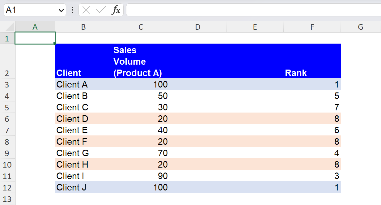
The following table contains client information (by client) as an example. The clients are given specific ranks based on their sales volumes. The formula in cell F3 in the table is as follows:
However, you can see the same ranks are given to numbers depending on whether there are duplicates. More specifically, Clients A and J are ranked in the first place, and Clients D, F, and H are assigned in the eighth position.

If you want to know how to break these ties, move on to the next section below.
How do you rank items based on multiple criteria or break ties in ranks with the RANK.EQ function?
Imagine that you want to keep the sales volume of Product A as a primary standard for client review but decide to add supplemental information, which is the sales amount for Product B. You can utilize the information as the second criterion to break ties in a ranking if any ties happen.
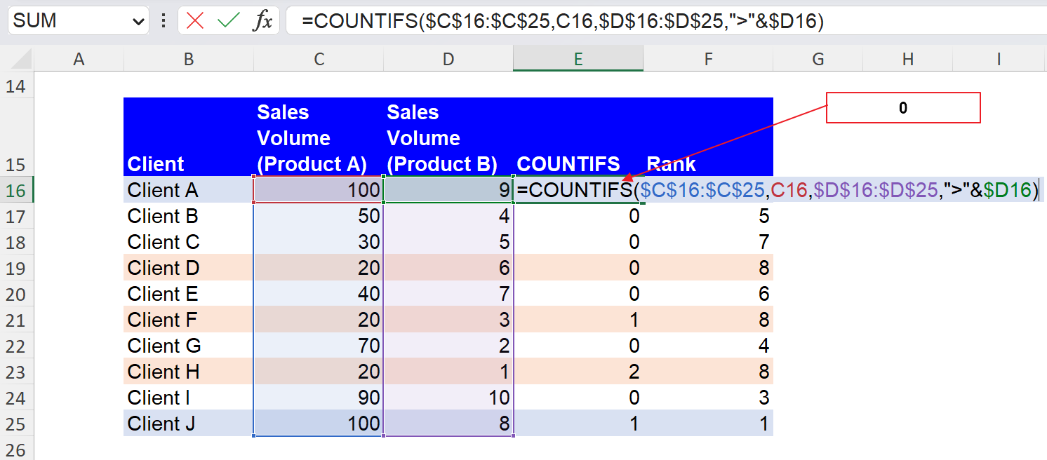
Here, you need to add a calculation for each client using the COUNTIFS function to give additional values to the computed rank and tweak the formula to compute the rank of each client. For example, the formula in cell E16 is as follows:
This formula returns the number of figures greater than a referred figure (9 in the screenshot below) in Column B only when its corresponding figure in Column A is repetitive in Column A. As you can see, Client A receives 0 from the COUNTIFS formula in Column E, while Client J earns 1 from COUNTIFS. You can see something similar happen to Clients D, F, and H - 0, 1, and 2 are given to each of them by the COUNTIFS function, respectively. These numbers provided by the COUNTIFS formula help determine the relative position of each client in the tied ranks.
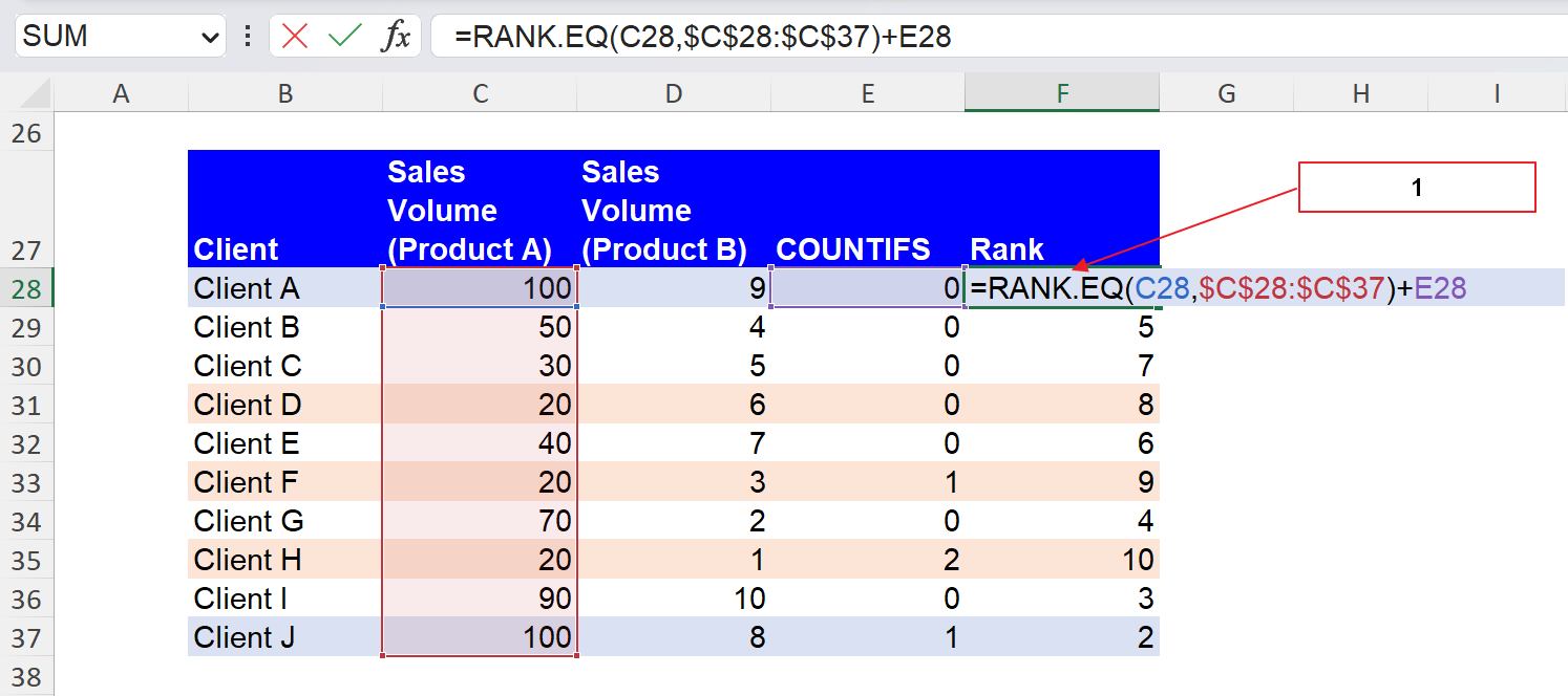
As the last step, you can compute the final rank by taking into account both the values provided by the RANK.EQ formula and ones calculated by the COUNTIFS function. You need to add up the two numbers, for example, as below:
You don’t see the same number repetitively in Column F. In this way, you can evaluate your clients primarily based on the sales volume of Product A without any tied ranks.
Although there are other approaches to solving this issue, we think this is one of the simplest approaches.
What is the difference between the RANK.EQ and RANK.AVG functions in Excel?
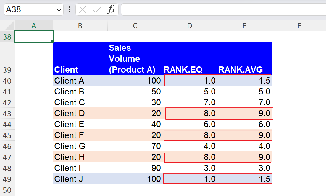
The RANK.EQ and RANK.AVG functions in Excel are similar but differ in handling ties in the dataset. The following picture helps you understand the difference visually.
When there are duplicate numbers,
- RANK.EQ assigns the top rank that one of the values occupied if they had a slightly different. In the case of the picture above, the formula gives 1 or 8 to tied sales volumes because Client A and J should be assigned to rank 1 or 2, and Client D, F, and H should be allocated to rank 8, 9, and 10.
- On the other hand, the RANK.AVG function gives the average rank available for the tied figures to each of them. In the example, the formula returns 1.5 or 9.0 to the same sales volumes as Client A and J should be assigned to rank 1 or 2, whose average is 1.5, and Client D, F, and H should be allocated to rank 8, 9, and 10, whose average is 9.0.
In summary, they give different numbers to tied figures while keeping their relative positions to the rest of the figures in a dataset.
Analyze your live financial data in a snap in Google Sheets
Are you learning this formula to visualize financial data, build a financial model, or conduct financial analysis? In that case, LiveFlow may help you automate manual workflows, update numbers in real-time, and save time. You can access various financial templates on our website, from the simple Income Statement to Multi-Currency Consolidated Financial Statement. Are you interested in this product but are an Excel user? That’s not a problem at all. You can connect Google Sheets to Excel quickly.
To learn more about LiveFlow, book a demo.

You can learn about other Excel and Google Sheets formulas and tips that are not mentioned here on this page: LiveFlow‘s How to Guides

