
RANK.AVG Function in Excel: Explained
In this article, you will learn how to use the RANK.AVG formula in Excel.
What does the RANK.AVG formula do in Excel?
The RANK.AVG formula in Excel returns the rank of a number in a dataset, with ties assigned an average rank. It is used to determine the relative position of a value within a range of values. For instance, if you have a series of integers, {1,2,3,4,5,5,7}, sorted in descending order, two of 5s are given rank 5.5, and number 7 is assigned to 7th place (not the sixth place).
When is it beneficial to use the RANK.AVG function in Excel?
The RANK.AVG function in Excel is beneficial when you need to rank a dataset and give the average rank to tied figures, not the top rank for the tied numeric values. In some datasets, it is common to have multiple values that are the same. As the RANK.AVG function assigns the average rank to the tied values, you can show a more moderate representation of the rank of each value, especially in large datasets where there may be many tied values.
How to use the RANK.AVG formula in Excel
The general syntax of the RANK.AVG function in as follows:
Here are the definitions of the arguments:
number: the number whose rank you want to find
ref: the entire range of cells containing the values to rank
order: an optional argument that specifies whether to rank the values in ascending or descending order. If this argument is omitted, the formula shows results in ascending order by default. When you enter a non-zero value in this argument, the formula also considers it in ascending order.
Note: The RANK.AVG formula assigns repetitive figures to the same position, affecting subsequent figures' ranks. For instance, in a series of integers, {3,2,2,1}, sorted in descending order, two of 2s are given rank 2.5, and number 1 is assigned to the 4th place (not the 3rd place).
The following sample table contains client information (by client). The customers are given specific ranks based on their sales volumes. The function in cell F3 in the table is as follows:
You can see the same ranks are given to numbers depending on whether there are duplicates. Clients A and J are ranked “1.5”, and Clients D, F, and H are assigned “9.0”.
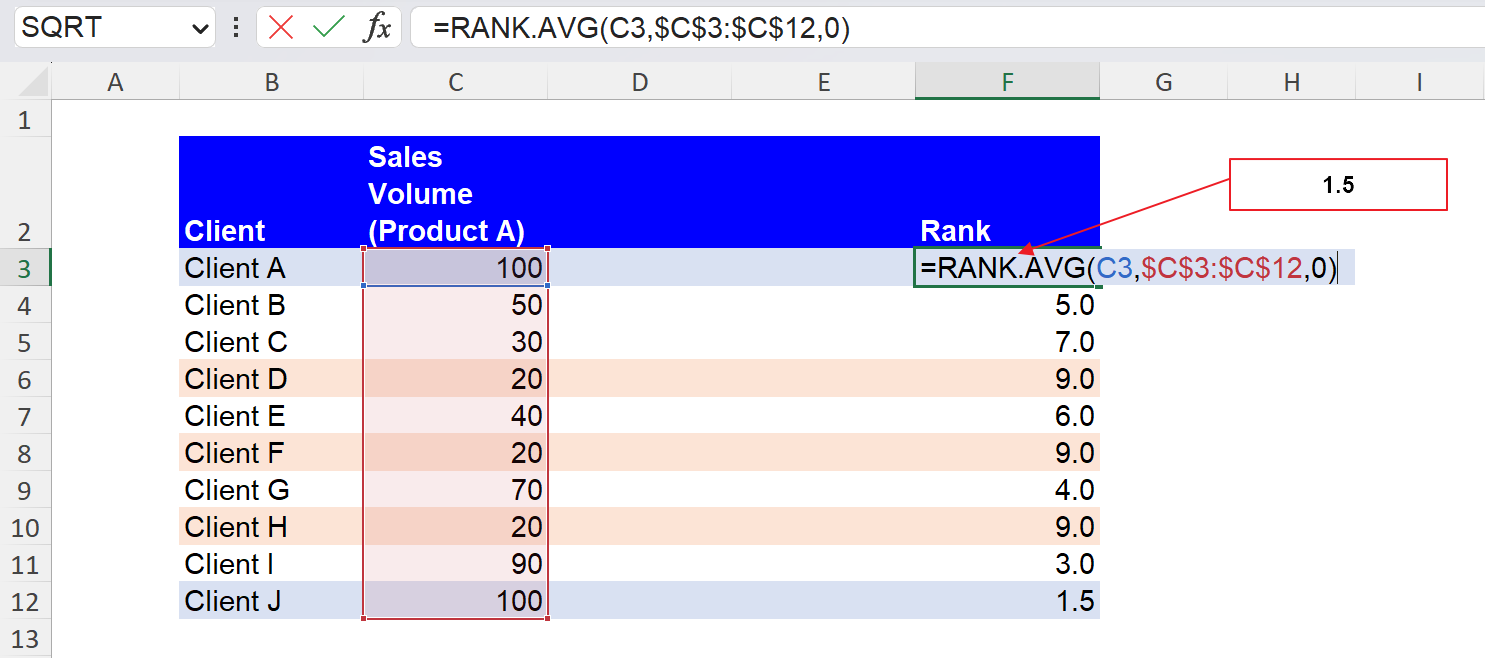
If you want to know how to break these ties, move on to the following section.
How do you rank items based on multiple criteria with the RANK.AVG formula?
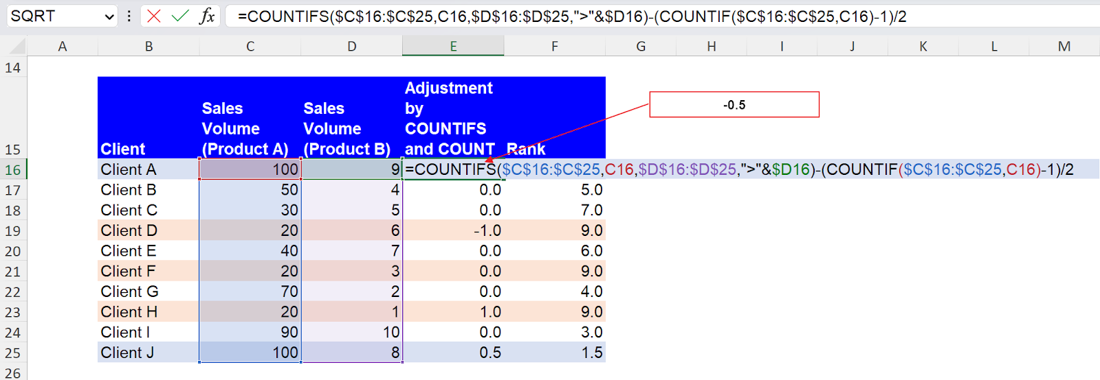
Suppose you want to use the sales volume of Product A as a primary criterion for client review and can add supplemental information, which is the sales amount for Product B. You can use the information as the second criterion to break ties in a ranking.

Here, you need to add Sales volume for Product B and adjustments for the ranking using the COUNTIFS and COUNT functions. For example, the formula in cell E16 is as follows:
This formula can be broken down into two parts as explained below:
The first half of the formula above returns the number of figures larger than a referred figure (9 in the screenshot below) in Column B only when its corresponding figure in Column A is repetitive in Column A. Client A receives 0 from this COUNTIFS formula, while Client J earns 1. These numbers provided by the COUNTIFS formula help determine the relative position of each client in the tied ranks.
Then, the second half of the formula above works as an adjuster to make the values from the COUNTIFS part into numeric values usable for ranking adjustment.
The entire long formula, including the COUNTIFS, COUNT, and other computations, gives you the numeric values to adjust the distance of each tied number from their average ranks so that all ranks are shown as integers. For example, the adjuster gives Clients A and J -0.5 and 0.5, respectively, as their average rank is 1.5.
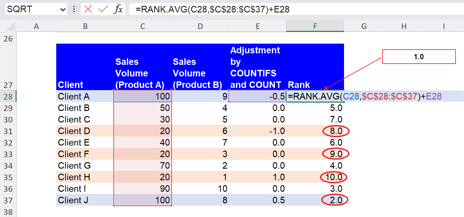
As the last step, you can calculate the final rank by taking into account both the values provided by the RANK.AVG formula and ones calculated by the adjustment formulas. You need to add them up, for example, as below:
You don’t see the same number repetitively in Column F. In this way, you can evaluate your clients primarily based on the sales volume of Product A without any tied ranks.
Although there are other approaches to solving this issue, we think this is one of the simplest approaches.
What is the difference between the RANK.AVG and RANK.EQ functions in Excel?
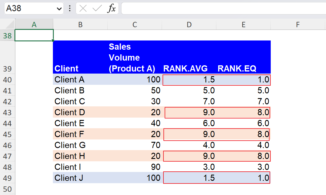
The RANK.AVG and RANK.EQ functions in Excel are similar but differ in handling ties in the dataset. The screenshot below allows you to understand the difference quickly.
When there are duplicate numbers,
- As described in this article, the RANK.AVG function provides the average rank available for the tied figures to each of them. In the example, the formula returns 1.5 or 9.0 to the same sales volumes as Client A and J should be assigned to rank 1 or 2, whose average is 1.5, and Client D, F, and H should be allocated to rank 8, 9, and 10, whose average is 9.0.
- In contrast, RANK.EQ assigns the top rank that one of the values occupied if they had a slightly different. In the case of the picture above, the formula gives 1 or 8 to tied sales volumes because Client A and J should be assigned to rank 1 or 2, and Client D, F, and H should be allocated to rank 8, 9, and 10.
In summary, they give different numbers to tied figures while keeping their relative positions to the rest of the figures in a dataset.
Analyze your live financial data in a snap in Google Sheets
Are you learning this formula to visualize financial data, build a financial model, or conduct financial analysis? In that case, LiveFlow may help you automate manual workflows, update numbers in real-time, and save time. You can access various financial templates on our website, from the simple Income Statement to Multi-Currency Consolidated Financial Statement. Are you interested in this product but are an Excel user? That’s not a problem at all. You can connect Google Sheets to Excel quickly.
To learn more about LiveFlow, book a demo.

You can learn about other Excel and Google Sheets formulas and tips that are not mentioned here on this page: LiveFlow‘s How to Guides


