AVERAGEIF Function in Excel: Explained
In this article, you will learn how to use the AVERAGEIF formula in Excel.
What is the AVERAGEIF formula in Excel?
The AVERAGEIF formula in Excel calculates the average of a range of cells that meet a specified condition.
When is it recommended to use the AVERAGEIF function in Excel?
The AVERAGEIF function in Excel is recommended when you want to compute the average of a range of cells that meet a particular criterion. It is useful when you want to find the average of a specific subset of the data from a large dataset. For example, if you have a sales data spreadsheet and want to calculate the average sales for a specific product, you can use the AVERAGEIF function to find the average of all sales for that product.
How do you use the AVERAGEIF function in Excel?
The general syntax for the formula is as follows:
"range" is the range of cells that you want to evaluate for the specified criteria.
"criteria" is the criterion that the cells in the range must meet to be included in the average.
"average_range" is an optional argument that allows you to specify a different range of cells to average. If you leave this parameter blank, the AVERAGEIF formula considers this argument the same as the “range” argument.
Note 1: If a dataset referenced for “average_range” contains blank cells, they are ignored when the formula computes the average. In case the “range”.
Note 2: The function returns #DIV! error value if “range” is a blank or a text value or if no cells in the selected range meet the conditions.
Note 3: Although the formula works even if the “range” and “average_range” are different sizes, it is highly recommended to include the same size of ranges for the two arguments.
How to use the AVERAGEIF formula with a numeric condition in Excel
Before looking at sample AVERAGEIF formulas containing numeric criteria, get yourself familiarized with logic operators, such as “>” (greater than) and “<” (less than).
- >N: Greater than N
- >=N: Greater than or equal to N
- <N: Less than N
- <=N: Less than or equal to N
- =N: Equal to N
- <>N: Not equal to N
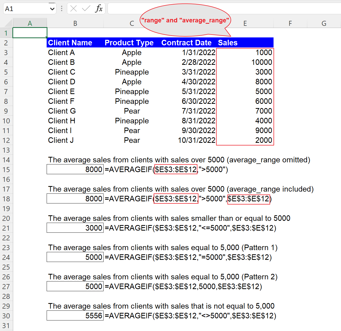
Assume you have the dataset in the picture below and want to compute the average sales amount that meets a specific criterion, such as the average sales from clients with sales over 5,000. The formula and its arguments are as follows:
=AVERAGEIF($E$3:$E$12,”>5000”,[$E$3:$E$12])
"range": $E$3:$E$12
"criteria": ”>5000”
"sum_range": $E$3:$E$12 (This is optional in this case)
You can see other examples in the screenshot below as well. Note that when you use an equal operator “=” with a specific number (the fourth example), you can directly input the particular number without the operator, as shown in the fifth example formula below.
How to use the AVERAGEIF function with a date criterion in Excel
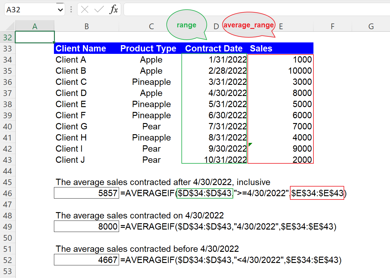
You can use a date as the “criteria” argument in the AVERAGEIF function, almost similar to a number criterion. So, you can combine a logic operator with a date to create a condition. However, note that you need to enclose a date with quotation marks when you directly enter it in the formula, such as the following formula:
"range": $D$34:$D$43
"criteria": ”>=4/30/2022”
"sum_range": $E$34:$E$43 (This can’t be omitted in this case)
.You can see two more sample formulas with date conditions in the following picture.
How to use the AVERAGEIF formula with a text condition in Excel
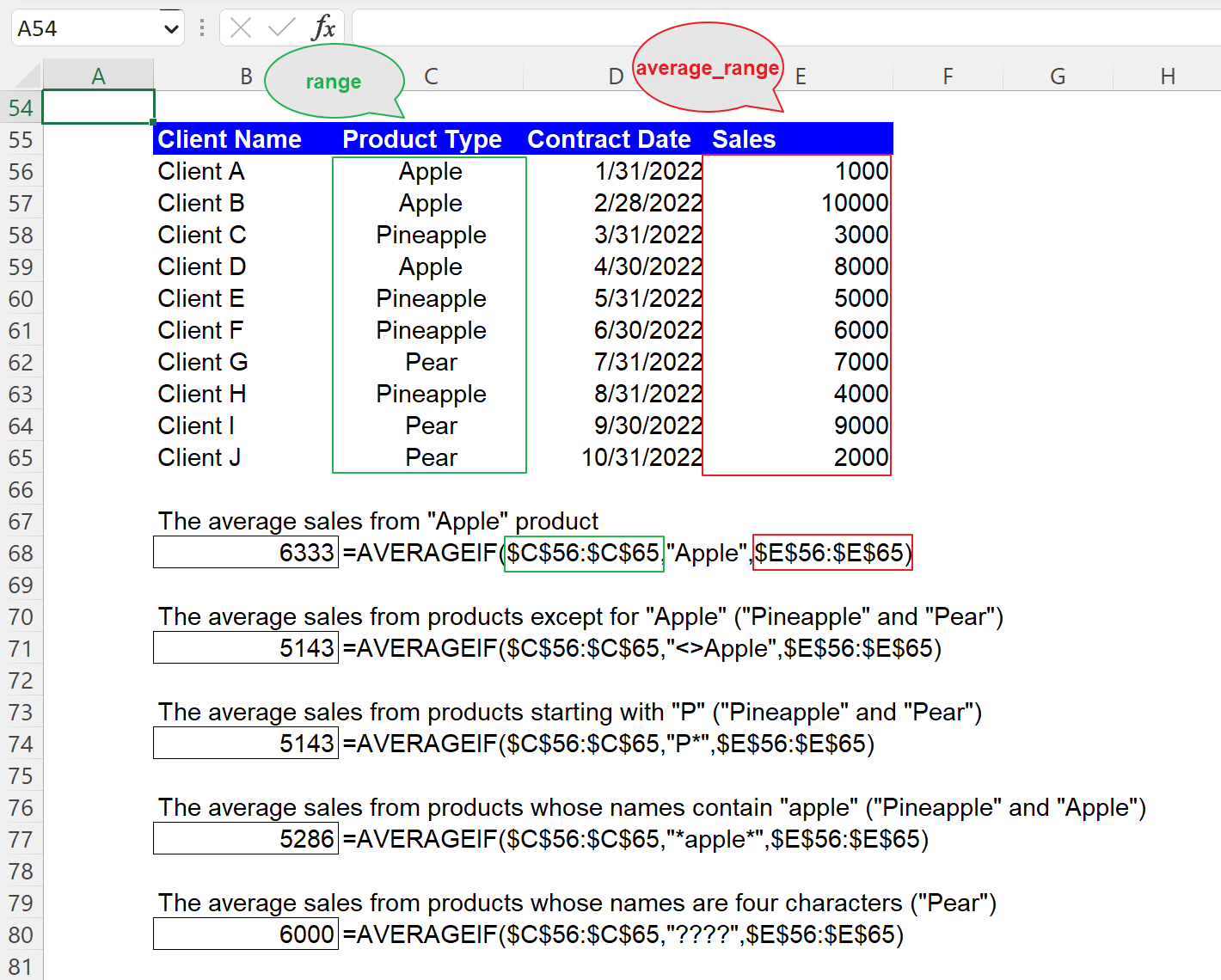
You must remember that when you manually insert a text condition as the “criteria” argument, you always need to enclose them with double quotes. Also, you can use the operators, such as “<>” or the wildcards, such as “*” and “?” together with a text string to form a condition. For instance, if you want to calculate the total sales amount from the product “Apple”, you can apply the following formula to the dataset.
"range": $C$56:$C$65
"criteria": ”Apple”
"sum_range": $E$56:$E$65 (This can’t be left blank in this case)
You should bear in mind that this formula is not case-sensitive. So, for example, you can get the same result when you use “apple” instead of “Apple” as “criteria” in the formula. The picture contains four more sample AVERAGEIF formulas with text conditions if you are interested.
How to use the AVERAGEIF formula with cell reference in Excel
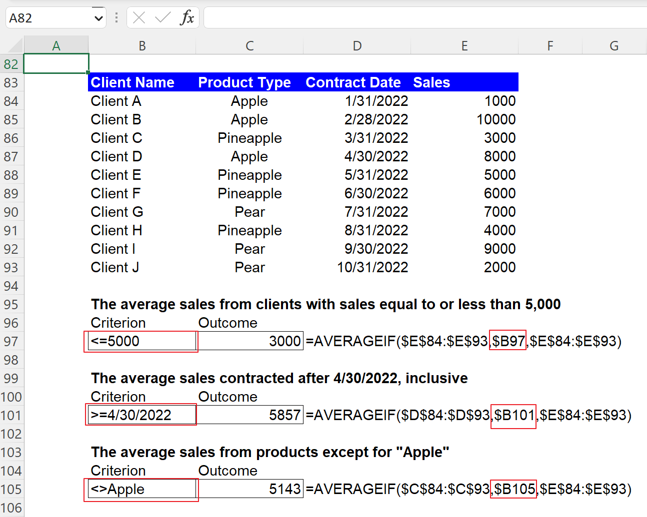
Although you can manually enter “criteria”, as shown in the examples above, instead, you can use the cell reference to input the “criteria” argument. We recommend the cell reference approach because it gives you more visibility and clarity about the condition as the requirement can be seen in a cell and allows you to change the condition more quickly. You don’t need to put your cursor on the cell containing the formula or open the cell by hitting the F2 button to see in detail or revise the function. Note that you don’t need to enclose it with quotation marks when you put a criterion in a cell, as shown in the picture below.
What is the difference between the AVERAGEIF and AVERAGEIFS functions in Excel?
The AVERAGEIF and AVERAGEIFS functions in Excel are similar in that they are both used to calculate the average of a range of cells that meet at least one criterion. However, the main difference is that the AVERAGEIFS function allows for multiple criteria, whereas the AVERAGEIF formula only allows for one requirement. So, you need to use the AVERAGEIFS formula when you want to apply more than one standard to your dataset and can use the AVERAGEIF function when you have only one criterion in your mind.
Analyze your live financial data in a snap in Google Sheets
Are you learning this formula to visualize financial data, build a financial model, or conduct financial analysis? In that case, LiveFlow may help you automate manual workflows, update numbers in real-time, and save time. You can access various financial templates on our website, from the simple Income Statement to Multi-Currency Consolidated Financial Statement. Are you interested in this product but are an Excel user? That’s not a problem at all. You can connect Google Sheets to Excel quickly.
To learn more about LiveFlow, book a demo.