XMATCH in Google Sheets: Explained
In this article, you will learn how to use the XMATCH function in Google Sheets.
What is the XMATCH function?
The XMATCH function is the enhanced MATCH function with more variety of search methods. Check this article if you want to know about the MATCH function.
How to use the XMATCH function in Google Sheets
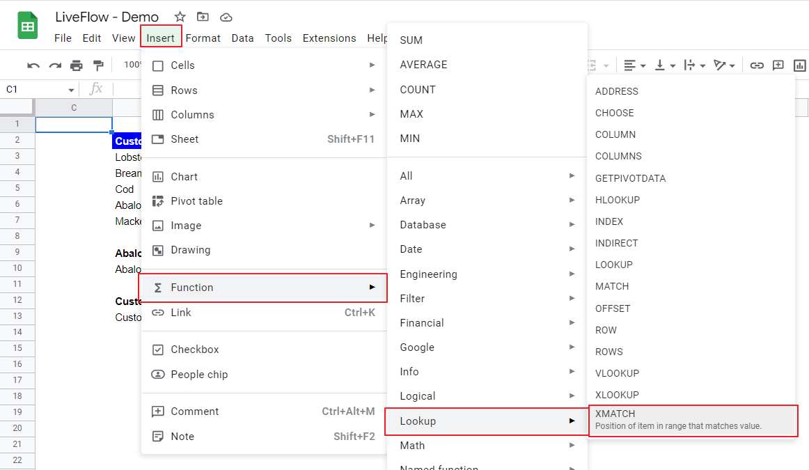
- Type “XMATCH” or go to “Insert” → “Function” → “Lookup” → “XMATCH”.
- Enter at least two arguments, “search_key” and “lookup_range” in the formula.
- Press the “Enter” key.
The general syntax of the formula is as follows:
Search_key: This is a value you want to know its position in a particular range.
Lookup_range: This is the range in which you look for the location of a specific value defined as “search_key”. This range should be a single column or row.
Match_mode (Optional): This value determines how the formula finds a match for the “search_key”.
0: With 0, the formula looks for an exact match.
1: The function looks for an exact match or the closest value larger than the “search_key”.
-1: The function works as a finder of an exact match or the closest value smaller than the “search_key”.
2: This allows the formula to look for a partial match. When you use this mode, the “search_key” should be a wildcard. Check this article on what a wildcard is.
Search_mode (Optional): This argument defines how the function searches the selected range for the target value.
1: If you choose one, the formula looks for a value from the first entry to the last one in the selected array.
-1: -1 works oppositely. It makes the function search for a value from the last entry to the first one.
2: With this number, the formula uses the binary search to find a value, assuming the range is sorted in descending order.
-2: With -2, the function applies the binary search method to reach a value, assuming the range is arranged in ascending order.
*If you are interested in what a wildcard is, check this article.
Look at the following example in which we run a vertical search with the XMATCH function.
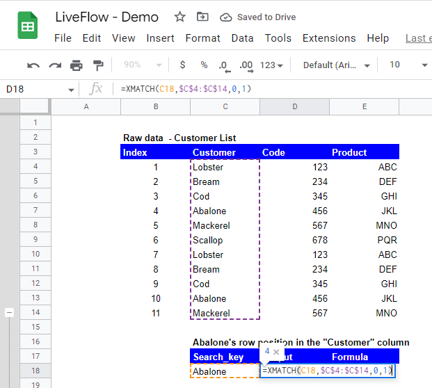
In this example, we input “Abalone” by cell reference as “search_key” and select a part of Column C, specifically C4:C14, as “lookup_range”. We input 0 and 1 for “match_mode” and “search_mode”, respectively. The formula looks for the position of “Abalone” in the selected array and returns “4” because “Abalone” is in the fourth row in the chosen area. It didn’t return “10” as the entered formula returns the first instance of “Abalone” which was specified as “1” under “search_mode”. For the formula to return “10”, the “search_mode” should be equal “-1”.
The following example shows a sample horizontal search.
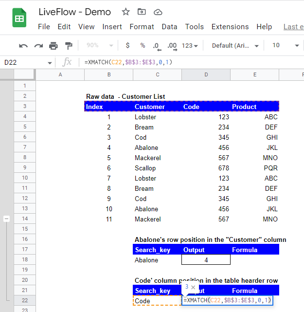
In this sample, we include “Code” by cell reference as “search_key” and select a part of Row 3, specifically B3:E3, as “lookup_range”. This is because we are trying to figure out where “Code” horizontally is. Similar to the first sample, we input 0 and 1 for “match_mode” and “search_mode”, respectively, as well. The formula looks for the position of “Code” in the selected row and returns “3” because “Code” is in the third column in the chosen area.
How “match_mode” and “search_mode” work in the formula
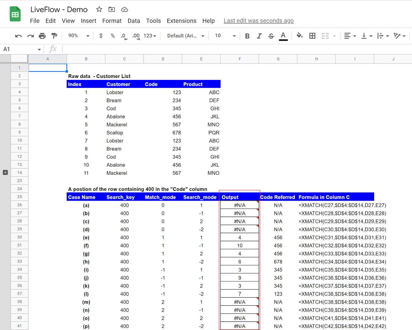
With the same sample data set, let’s figure out how the formula works differently depending on “match_mode” and “search_mode”. As each of “match_mode” and “search_mode” has four patterns, there are sixteen (=four multiplied by four) types of combinations. See cases from (a) through (p). The “Output” column shows the returns from the XMATCH formulas. You can quickly realize that they are significantly different.
(i) Cases (a) to (d)
In these cases, the XMATCH formulas do not work because there is no value that exactly matches 400 in the selected range.
(ii) Case (e)
As the “match_mode” is “1”, the formula looks for 400 or a value closest to and larger than 400 (This principle applied to the subsequent three cases, Case (f) to (h) as well). Then, as the “search_mode” is “1”, the formula searches the range from top to bottom for the value. The value that meets these principles is “456”, the fourth value in the selected range; the formula returns “4”.
(iii) Case (f)
The only difference between this case and Case (e) is the “search_mode”. This time the formula tries to seek the array from bottom to top for the value. As there is another “456” in the 10th row in the chosen range, the function returns “10”.
(iv) Case (g)
The only difference between this case and the previous two is, again, the “search_mode”. In this case, the formula runs a binary search; it tests “400” against the value in the middle of the selected data set, which is “678”. Then, as the formula assumes the range is sorted in ascending order, it judges that the value the formula is looking for locates above “678”. Thus, the function pulls out “4”, which is the position of “456” sitting in the fourth row of the selected range.
(v) Case (h)
This case is similar to Case (g). The difference is that the formula runs a binary search, assuming the selected array is arranged in descending order. So, in this case, the formula tries to find the value it is seeking below “678”. However, the problem is there is “123” right beneath “678”, the formula judges “678” as the value nearest to “400” and gives “6” as a return, without looking at other numbers under “123” given the assumption that the data is sorted in descending order.
(vi) Case (i) through (l)
These cases have “-1” as “match_mode” so the formulas try to find the value nearest and smaller than “456”. With this assumption in your mind, look at cases (ii) to (v) to understand how different “search_mode” affects the result of the XMATCH function and why the formula returns different values in cases (i) to (l).
(vii) Case (m) to (p)
These formulas are not working because their “match_mode” is “2”, which is for a wildcard match. As the given search_key of “400” is not a wildcard, the formulas do not work correctly.
What you learn from these cases is that “match_mode” and “search_mode” change the return of the formula significantly, depending on their setting, so you should be careful when you try to search a complex data set (e.g., one has duplication in items) for a specific value. We highly recommend that you organize and streamline the data set as much as possible and use the simple and clear combination of “march_mode” and “search_mode” such as “0” and “1”.
What does XMATCH return if there is no match?
When the XMATCH doesn’t find any match, it returns “#N/A”. If this happens, you need to review your “search_key” and/or “lookup_range” and revise the arguments appropriately.
How does MATCH function work in Google Sheets?
The MATCH formula works similarly to the XMATCH function but with limited search options, which we think are enough for general information search in a data set. Read this article to learn the MATCH function in Google Sheets.
Is there an alternative to XMATCH?
The combination of INDEX and MATCH functions can be one of the alternatives. Check this article to learn how to use INDEX/MATCH in Google Sheets.

