How to Use INDEX Function in Google Sheets
In this article, you will learn how to utilize the INDEX function in Google Sheets. This function is beneficial when you want to pull out values in a row, a column or an array, or a value in a cell.
How to Use the INDEX formula in Google Sheets
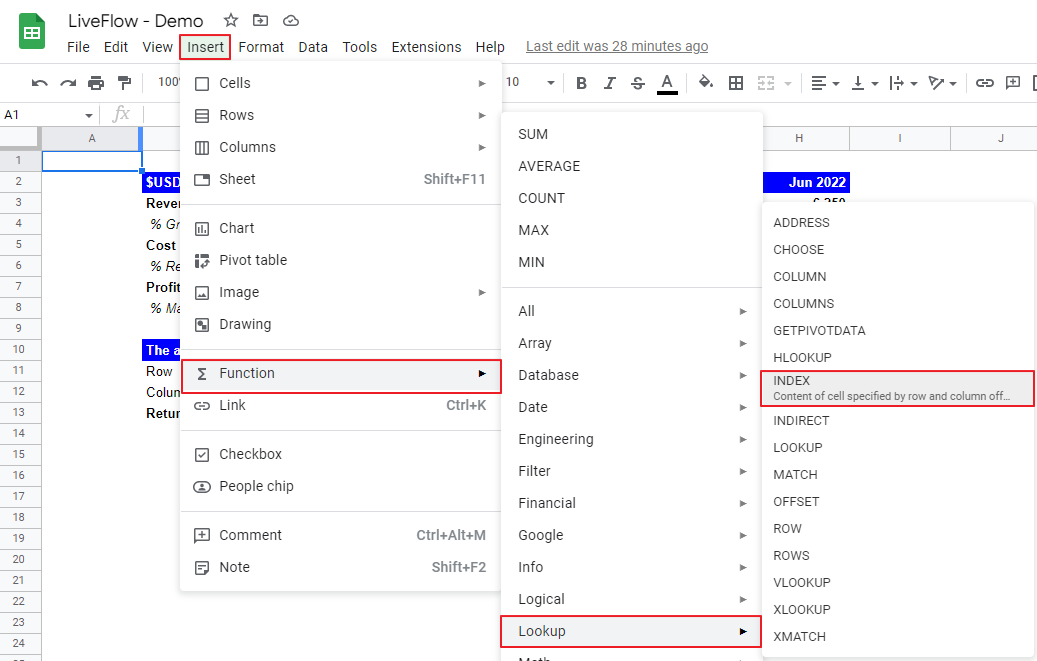
- Type “=INDEX” or go to “Insert” → “Function” → “Lookup” → “INDEX”.
- Input a “reference”, a range from which you want to pull out information
- Enter the address of the target value(s) by inputting “row” and “column”, if necessary
The generic formula is as follows:
This function is beneficial if you want to find a relative position of an item in a particular range.
Reference: This is the range from which any values are returned by the formula.
[Row]: This is an optional input. The relative index number of the row within the “reference” from which the value(s) is returned
[Column]: This is an optional input as well. The relative index number of the column within the “reference” from which the value(s) is returned.
If you enter
(i) nothing for both “row” and “column”, the formula returns all values in the selected range in “reference”;
(ii) only “row”, the function returns all cell values in a row in the chosen array as “reference”;
(iii)only “column”, the function returns all cell values in a column in the chosen array as “reference”; and
(iv) both “row” and “column”, a value in a cell that is an intersection of “row” and “column”.
If you want to get a single specific value from this formula, the important prerequisite is knowing where the value is in terms of the row and column numbers in the selected range.
Assume you are a manager in the Finance Group in your company. You are checking a financial data set for the six months. You want to pull out the % Margin of Profit in March 2022. Luckily, you know the cell’s address, the seventh row, and the fourth column in the chosen range.
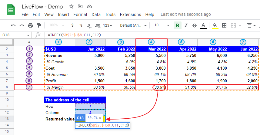
Reference: $B$2:$H$8 - It is typical to select the entire data set, including a row for table headers and a column for item names.
[Row]: 7 - This is not Google Sheets’ row index but the relative row number in the selected range.
[Column] 4 - Same as “row”, this number is not for Google Sheets’ column index but the relative column number in the chosen field.
As a result, the function returns the value at the intersection, which is 30.9%.
Think about what you would get as an outcome of the formula if you don’t fully input the address in the function. You will get
(i) the entire table (values in B2:H8) if you enter none of “row” or “column”;
(ii) the entire seventh row when you enter only “row” number (7) in the formula; or
(iii) the entire fourth column if you enter only “column” number (4) in the formula.
How do I use INDEX and MATCH functions together in Google Sheets?
The INDEX formula is useful when you know the address of the value you want to see. However, in many cases, in reality, you don’t know the exact location of the value you want to show, though you have a clue or a keyword such as “% Margin” and “Mar 2022”.
In such a case, you can still use the INDEX function by incorporating the MATCH function. Check this article to learn how to use the INDEX and MATCH functions together with a practical example.

