
How to Use VLOOKUP in Google Sheets
In this article, you will learn how to use the VLOOKUP formula in Google Sheets.
This function is beneficial when you need to extract necessary information out of a table containing lots of irrelevant items and data. Its function is to search for a specific value in a column and return a value in a different column in the same row.
How to use the VLOOKUP formula in Google Sheets
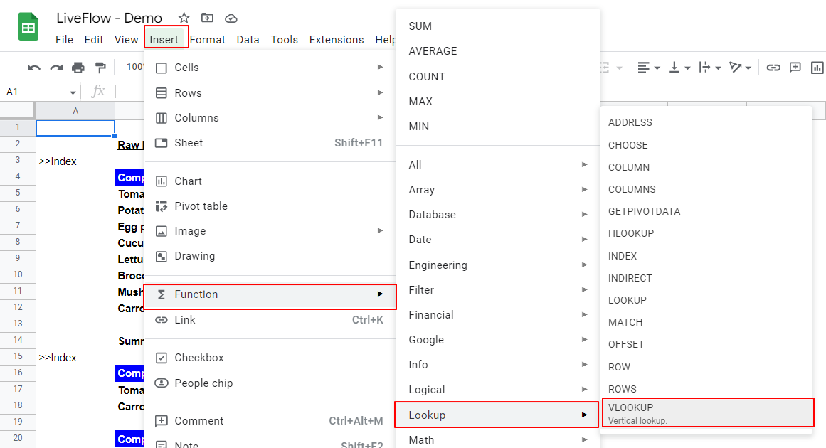
- Type “=VLOOKUP(” or go to “Insert” → “Function” → “Lookup” → “VLOOKUP”
- Select “Search_key”, specify “Range”, input “Index”, and enter “FALSE” or “TRUE”.
Generic formula
Search_key: This is a value based on which this formula looks for a specific item.
Range: This is the entire area within which this function looks for a specific item. The leftmost column should contain a particular keyword you enter as search_key.
Index: This is the position of a column within the range selected from which the formula pulls out requested information. For example, if the specified range is C5:E9 and you want to see the data in Column D, this index number should be 2, as Column D is the second column in the chosen field.
[is_sorted]: You need to choose “FALSE” for an exact match or “TRUE” for the closest match. You can leave this part blank but in this case it is taken as “TRUE”. So, you are recommended to enter “FALSE” to avoid pulling out incorrect data.
Learn how it works by looking at the example below. Assume you are a customer relationship manager, you have a set of data, Raw Data in the picture below, and you need to extract the revenue of an Eggplant company.

- The “search_key” should be “Eggplant” as you look for data relevant to Eggplant in B14.
- Then, the “range” should include at least the column including “search_key” as the leftmost column, and also the one containing the data you want to know, in this case, the column showing “Revenue”. In this example, we select the entire table as “range” - $B$5:$I$9.
- The next step is to enter “index” in the formula. You need to be aware that the index count starts from the leftmost column and counts as one. So, in the sample table, the column's index incorporating revenue data is 6. For your visibility, we show the index of each column in the third row. We recommend you do this, give an index number to a column and make it visible once the “range” is fixed in the cell C12.
- Finally, enter “FALSE” or “TRUE” or keep it blank, which is considered “TRUE”. The “FALSE” allows only values that exactly match the search_key. The “TRUE” extracts the nearest values to the "search_key". As “TRUE” may not bring the correct answers, we recommend you always use “FALSE”. See two examples below of how they work.
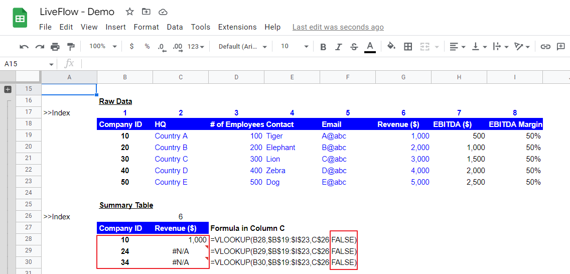
At the bottom part of the upper screenshot, you can see two “#N/A” next to the company IDs of “24” and “34”. This is because there is no figure that exactly matches them in the leftmost column in the selected range, specifically, B:19 through B:23, {10,20,30,40,50}.
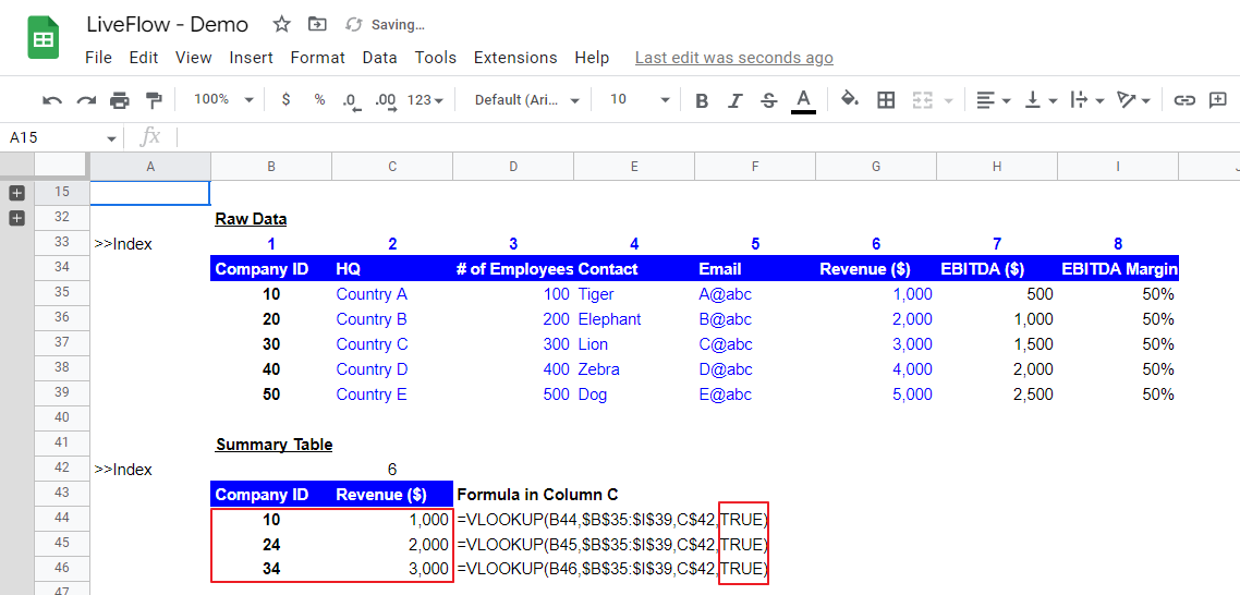
However, if you use “TRUE”, as you observe at the bottom part of the second screenshot below, values are returned by the formulas even if the company IDs of 24 or 34 do not exist in the raw data.
How do I VLOOKUP from one sheet to another in Google Sheets?
You may have a table containing copious data in a separate tab and want to make a summary table in another tab. You can refer to data on a different sheet by going there while you select “range” in the formula.
Check this article: How to Reference Another Sheet in Google Sheets, if you don’t know how to go to another worksheet while selecting a range.
Why doesn’t VLOOKUP work in Google Sheets?
The major mistakes and causes of errors when you use the VLOOKUP are as follows:
- The column that should contain a “search_key” is not the leftmost or is not included in the selected range.
- The range you select does not contain the column from which you want to excerpt data.
- You enter “FALSE” in the VLOOKUP formula but its “search_key” doesn’t exist in the raw data like shared in the example above.
- The formula's index number is incorrect after inserting a column(s) in the raw data table. The index number should be double-checked and updated if you make any changes to the raw data table.
- There is more than one value that matches search_key in the raw data. In this case, the formula typically returns only a value of the first match and doesn’t return other matches. You need to ensure that you don’t have duplication in the column for search_key in the selected “range”.
- There is a typo(s) in your “search_key”. You should avoid the manual input of “search_key” as much as possible.
What is the alternative for VLOOKUP?
If you are looking for an alternative method of the VLOOKUP formula, we can suggest you use a combination of INDEX and MATCH functions. If you have never tried the functions, you should learn them because they are more flexible than the VLOOKUP function.
Check this page to understand how to use these functions. Other alternatives could be XLOOKUP and HLOOKUP, depending on your dataset and what type of search you want to do.


