
How to Use HLOOKUP in Google Sheets
In this article, you will learn how to use the HLOOKUP formula in Google Sheets.
This function is beneficial when you need to extract necessary information out of a data set containing lots of irrelevant items. Its function is to sort for a specific value in a row and return a value in a different row in the same column.
How to use the HLOOKUP formula in Google Sheets
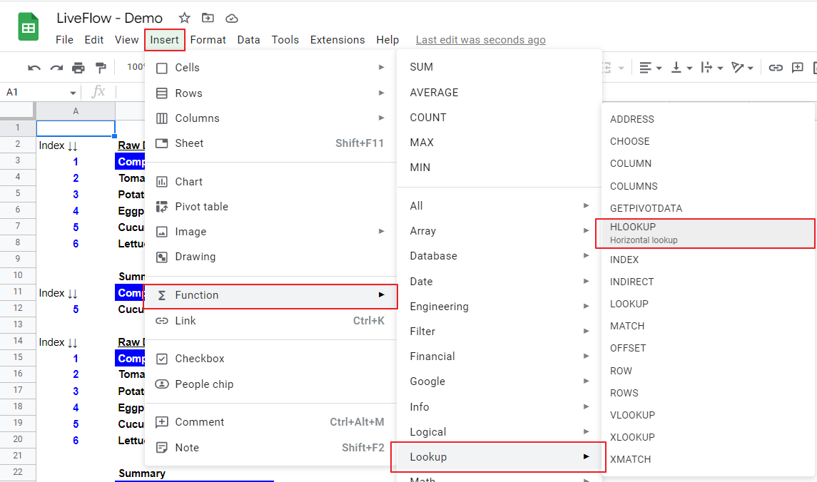
- Type “=HLOOKUP(” or go to “Insert” → “Function” → “Lookup” → “HLOOKUP”.
- Select “Search_key”, specify “Range”, input “Index”, and enter “FALSE” or “TRUE”.
Generic formula
Search_key: This is a value based on which this formula looks for a specific item.
Range: This is the entire area within which this function looks for a specific item. The uppermost row should contain a particular keyword you enter as search_key.
Index: This is the position of a row within the range selected from which the formula pulls out requested information. For example, if the specified range is C5:E9 and you want to see the data in Row 6, this index number should be 2, as Row 6 is the second row in the chosen field.
[is_sorted]: You need to choose “FALSE” for an exact match or “TRUE” for the nearest match. You can leave this section blank, but it is taken as “TRUE” in this case. So, you are recommended to enter “FALSE” to avoid pulling out incorrect data.
Learn how it works by looking at the example below. Assume you are a finance manager, you have monthly revenue data by client, Raw Data in the picture below, and you need to sort a revenue amount from Cucumber Company in April 2022.

- The “search_key” should be “April 2022” and the formula goes down to the bottom by the number of “index” you are going to enter.
- Then, the “range” should include at least the row including “search_key” as the top row, and also the one containing the data you want to know, in this case, the row showing Cocumber’s data - row 8. In this example, we select the entire table as “range” - $B$3:$H$8.
- The next step is to enter “index” in the formula. You must be aware that the index count starts from the topmost row and counts as one. So, in the sample table, the row's index incorporating Cucumber data is 5. For your visibility, we show the index of each column in Column A. We recommend you give an index number to a row and make it visible once the “range” is fixed in cell C12.
- Finally, enter “FALSE” or “TRUE” or keep it blank, which is considered “TRUE”. The “FALSE” allows only values that exactly match the "search_key". The “TRUE” extracts the closest values to the search_key. As “TRUE” may not bring the correct answers, we recommend you always use “FALSE”. See two examples below of how they work.
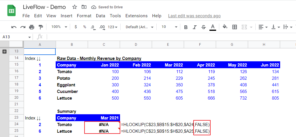
Assume you made a mistake in “search_key” and you entered “Mar 2021”, which should be “April 2022”. At the bottom part of the upper screenshot, you can see two “#N/A” next to the company names of “Tomato” and “Lettuce”.
This is because there is no period that exactly matches “Mar 2021” in the topmost row in the selected range, precisely, B:15 through H:15, {Company, Jan 2022, Feb 2022, Mar 2022, Apr 2022, May 2022, Jun 2022}.
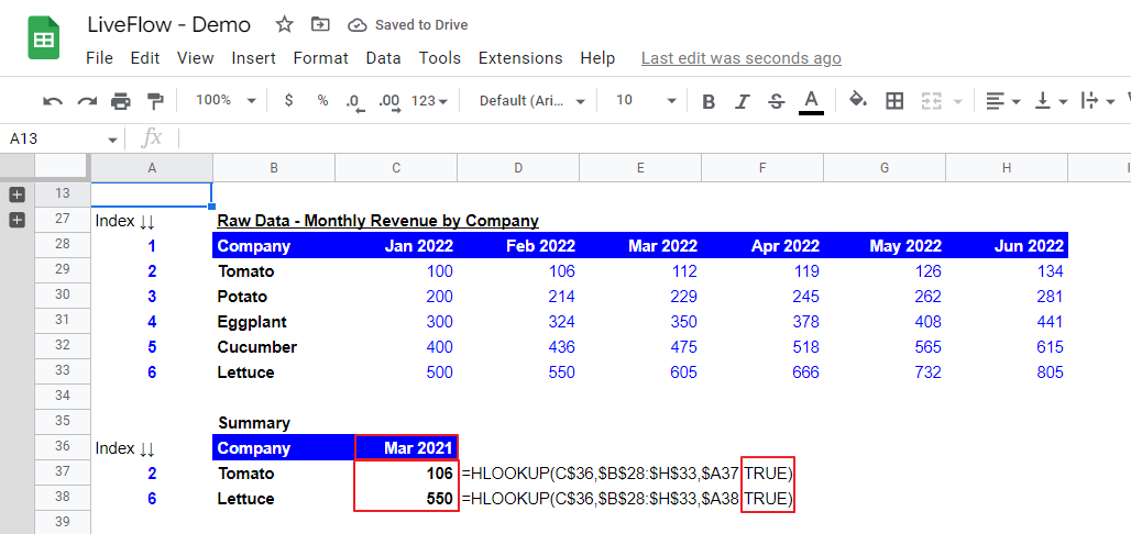
However, if you use “TRUE”, as you observe at the bottom part of the second screenshot below, values are returned by the formulas even if “Mar 2021” does not exist in the raw data.
Why doesn’t HLOOKUP work in Google Sheets?
The major mistakes and causes of errors when you use the HLOOKUP are as follows:
- The row that should contain a “search_key” is not at the top or is not included in the selected range.
- The range you select does not contain the row from which you want to excerpt data.
- You enter “FALSE” in the HLOOKUP formula, but its “search_key” doesn’t exist in the raw data as shared in the example above.
- The formula's index number is incorrect after inserting a row(s) in the raw data table. The index number should be double-checked and updated if you make any changes to the raw data table.
- There is more than one value that matches search_key in the raw data. In this case, the formula typically returns only a value of the first match and doesn’t return other matches. You need to ensure that you don’t have duplication in the row for search_key in the selected “range”.
- There is a typo(s) in your “search_key”. You should avoid the manual input of “search_key” as much as possible.
What's the difference between VLOOKUP and Hlookup?
The VLOOKUP formula is often used to find an item on a vertically long table, whereas the HLOOKUP function is usually used to sort data on a horizontally long table.
The significant difference is, that the VLOOKUP formula searched the leftmost column for “search_key” while the HLOOKUP function seeks “search_key” for the topmost column in each selected range.
How do I use VLOOKUP in Google Sheets?
Read this article if you are interested in how to use the VLOOKUP function in Google Sheets.
How do I use VLOOKUP and HLOOKUP together?
There are two patterns of formula - (i) the HLOOKUP function in the VLOOKUP formula and (ii) the VLOOK function in the HLOOKUP formula. To combine the VLOOKUP and HLOOKUP functions, you need to tweak the data table in which you want to find specific data. See example formulas in the screenshots below.
The third example shows the combination of INDEX and MATCH functions, which is the alternative to the combination of VLOOKUP and HLOOKUP formulas.
(i) The HLOOKUP function in the VLOOKUP formula
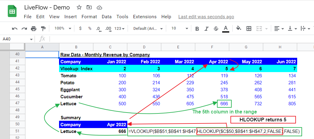
In this example, the HLOOKUP is used to find a number, which is included in the VLOOKUP formula as “index”.
As the HLOOKUP function can search data only downwards under the uppermost column, it is ideal that its target row (in this case, “Vlookup:Index”) is the second row, right beneath the top row in the selected field to minimize the format change of the data table.
As the HLOOKUP returns 5, which is in the second row in the “Apr 2022” column within the selected area, the VLOOKUP formula looks for the 5th column in the row named “Lettuce”, which returns “666”, as you can see.
(ii) The VLOOKUP function in the HLOOKUP formula
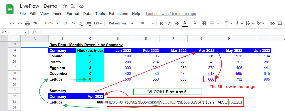
In the second example, similar to the first formula, the VLOOKUP formula works as an index number finder for the HLOOKUP formula.
As a preparation, you should insert an additional column for HLOOKUP’s index number next to the “Company” column to the right because the VLOOKUP formula can search data right from the leftmost column. The VLOOKUP function returns 6 in the second column in the “Lettuce” row as the index number in the VLOOKUP is 2.
Then, the HLOOKUP finds “666”, located in the 6th row in the “Apr 2022” column within the selected field.
What is the alternative for HLOOKUP?
If you are looking for an alternative method of the HLOOKUP formula, we can suggest you use a combination of INDEX and MATCH functions. If you have never tried the functions, you should learn them because they are more flexible than the HLOOKUP function.
Also, the XLOOKUP would be another option. Read this article for your understanding of the XLOOKUP function: XLOOKUP - Google Sheets: Explained
Here’s a quick explanation of INDEX and MATCH. Check this page to understand how to use these functions.
The combination of INDEX and MATCH functions

In this combination of the INDEX and MATCH functions, the MATCH functions work as pathfinders for the INDEX formula. The INDEX formula needs an input of the entire range where we are looking for a solution, so we will index the full table.
The top row and left column are counted as first ones in a selected array. In the example above, the first MATCH gives where the target row is, and the second MATCH brings where the target column is to the INDEXfunction. With these values, the INDEX function gets the specific coordinate of the target value.
The major benefits of this combination, compared to the combination of the VLOOKUP and HLOOKUP, are:
1. You can apply the formulas to the existing table without adjusting the data table (e.g., inserting a new column or row for indexes of the formulas).
2. You don‘t need to make any changes to the formula when you make adjustments to the table, such as inserting new columns and rows for new information or a set of additional data, as long as the adjustments are made in the selected array in the formulas.


