
COLUMN Function in Google Sheets: Explained
In this article, you will learn how to use the COLUMN function in Google Sheets. The COLUMN function simply returns the column number of a particular cell.
How to use the COLUMN formula in Google Sheets
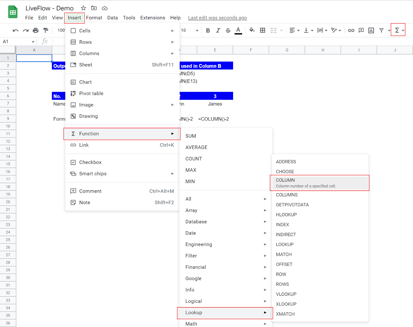
- Type “=COLUMN(” or go to “Insert” → “Function” (or directly navigate to the “Functions” icon) → “Lookup” → “COLUMN”.
- Input a specific cell by cell reference or manual input, or leave the argument blank.
- Press the “Enter” key.
The general syntax is as follows:
Cell_reference[Optional]: You can refer to a cell. The formula returns its column number.
Note: If you leave the argument blank, the function returns the column number of the cell in which it is located. For example, if you insert the COLUMN function in cell B4 and keep the parameter unfilled, the formula returns “2” as the formula is in the second column. Also, even if you don’t fill in the argument, you still need to input “()”, parenthesizes.
Look at the following examples.

The upper table shows two examples in which you refer to a cell in the COLUMN function. In the first example, as the function refers to cell D5, the formula returns 4, which is the column number of the cell referred to (D is equivalent to 4).
The lower table presents the sample table using the column function for its number of items (Row 6). As you can see, you can get a series of consecutive numbers starting from 1 by entering a formula like “COLUMN() - X”. X should be the number that makes the formula COLUMN()-X equal to 1. In this example, as the first item, Sam, is in cell C7, you should enter “=COLUMN()-2” in cell C6 and copy and paste it to other cells in the same row.
What does a column mean in Google Sheets?
A column is a vertical set of cells. A row is a horizontal series of cells.
How do I refer to a column in Google Sheets?
You can refer to a column range by simply selecting the range when you are inputting an argument for a formula. If you want to select the entire column, you can input its column index twice with a colon between the indexes, such as “=SUM(B:B)”, which aggregates all numbers in Column B.


