How to Use CHOOSE Function in Google Sheets

In this article, you will learn how to utilize the CHOOSE formula in Google Sheets. The CHOOSE function is suitable when you conduct a scenario analysis in which you need to change a value in a cell depending on the scenario you select.

‍

How to use the CHOOSE formula in Google Sheets

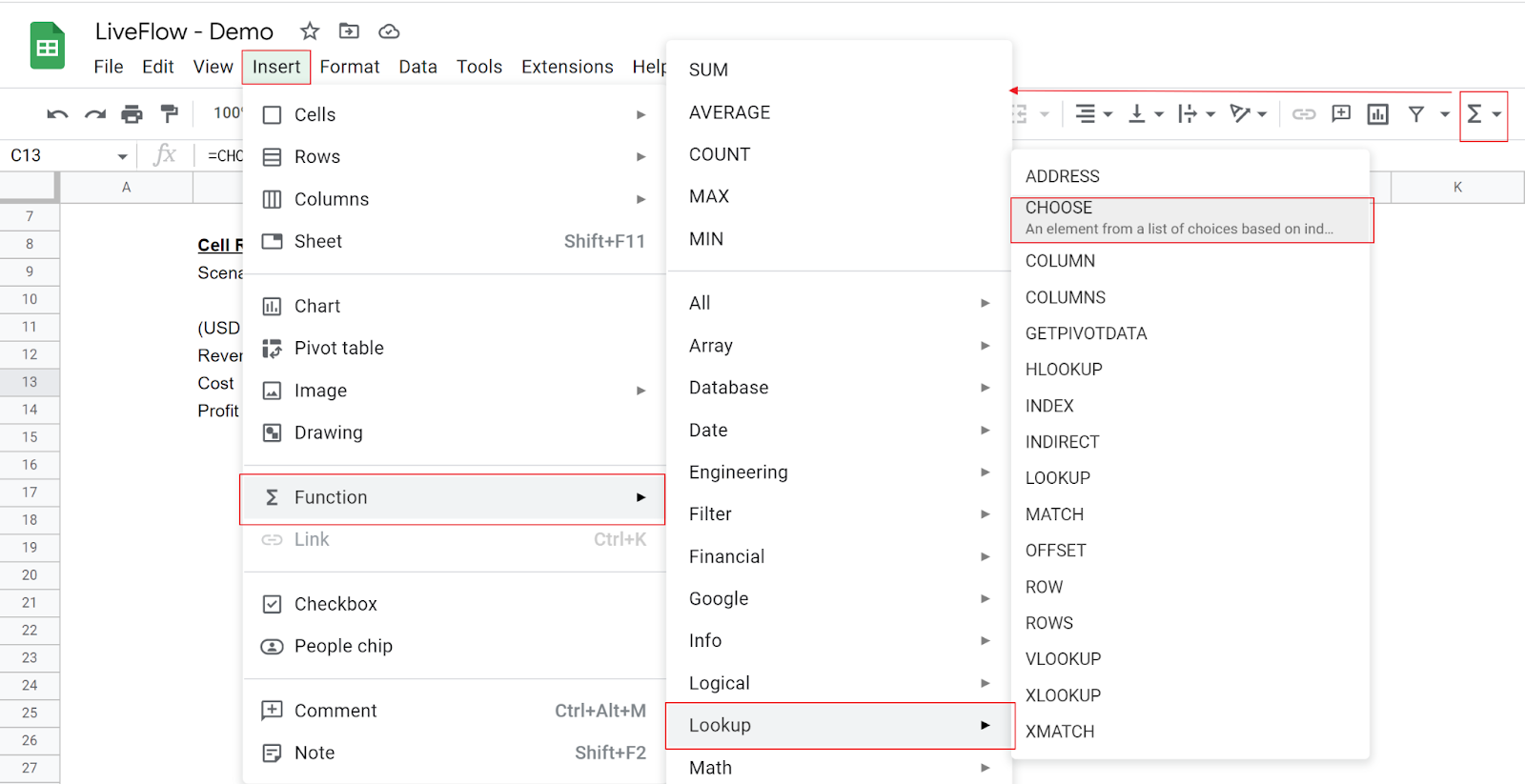
1. Type “=CHOOSE(” or navigate to the “Insert” tab (or “Functions” icon) → “Function” → “Lookup” → “CHOOSE”.
2. Enter “start_date” and “months” by manual input or cell reference.
3. Press the “Enter” key.

‍

The general syntax is as follows:

=CHOOSE(index, choice1, [choice2, …])

Index: The value for this parameter should be a number from one up to twenty-nine (inclusive).

Choice1: This is the output value corresponding to the “index” of “1”.
Choice2: This is the value shown when the “index” is “2”.

Note: you need to input as many choices as the number of scenarios you have. For example, if you have three scenarios and the “index” can be one of the integers from one to three, you need to enter choices - “choice1”, “choice2”, and “choice3” in the formula.

‍

The CHOOSE formula is effective when you conduct scenario analysis and want to keep the entire structure and the existing numbers unchanged because the function allows you to replace a value with another value depending on the case you choose. You can leverage what you build for a scenario for other scenarios by using the CHOOSE formula; You don’t need to replicate unchanged parts to analyze the other cases.

‍

Assume you are a finance manager and want to check how much your company’s profit changes if the cost varies. You assume three scenarios: (i) the cost is $500mm, (ii) it is $750mm, and (iii) it is $1,000mm. What you are recommended to do is as follows:

1. Prepare a cell for scenario input (cell C9 in the picture).
2. Create a simple table and input “Revenue” and “Profit” and their numbers - let’s assume revenue is $1,000mm and fixed. Profit should be the result of “Revenue” less “Cost” (=C12-C13)
3. Enter three cost numbers in the row in which the “Cost” is shown, Row 13, and give them headers such as “Scenario 1” as shown in the screenshot.
4. Finally, enter the CHOOSE formula in cell C13, and refer to cell C9 as the “index” and cells E13, F13, and G13 from left to right for “Choices 1-3”.
5. If you want to switch the case, change the number in cell C9 within the range of 1 to 3. You can see different “Profit”.

‍

We highly recommend that you use cell references for the CHOOSE formula because it

1. allows you to quickly check which scenario is chosen without opening the formula;
2. gives you visibility on scenario numbers - the “Cost” in this case; and 
3. lets you change by typing different figures in cell E13, F13, or G13, without revising the formula itself.