ISNA Function in Google Sheets: Explained

‍

In this article, you will learn about the ISNA function in Google Sheets and how to effectively use it for error handling.

‍

‍

What is the ISNA function in Google Sheets?

‍

The ISNA function in Google Sheets is used to check whether a specific value or a formula result returns the #N/A error.

‍

The #N/A error indicates that the value being looked up or referenced is not available or not found. The ISNA function returns TRUE or FALSE as the output.

‍

‍

‍

Uses of ISNA function in Google Sheets

‍

The ISNA function in Google Sheets is primarily employed for error handling and data validation purposes. Some common applications include:

‍

• Checking for #N/A errors: Identify cells with #N/A errors and take appropriate actions, such as replacing the error with a value or modifying the formula to avoid the error.

‍

• Nested formulas: Combine ISNA with other functions like IF and IFERROR to create more complex formulas. For instance, test whether a VLOOKUP or INDEX formula returns an #N/A error and return a specific value or message if it does.

‍

• Data validation: Use ISNA in data validation rules to ensure users enter valid data. Set up rules that require users to input values not equal to #N/A in specific cells or ranges.

‍

‍

How to use the ISNA formula in Google Sheets

‍

The formula is as follows:

=ISNA(value)

‍

Where value is the cell or range of cells you want to check.

‍

• Select the cell where you want to display the outcome.

‍

• Enter the following formula into the cell: =ISNA(

‍

• Enter the value after the open parenthesis and then close the parenthesis.

‍

‍

‍

Sample use case for ISNA function in Google Sheets

‍

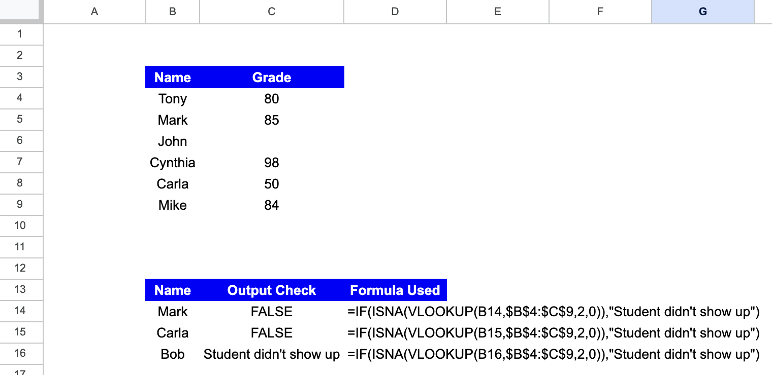
Suppose you have a list of students with their scores in a particular paper, and you want to cross-check against a separate list to identify which students did not show up for the exam.

‍

A combination of IF, VLOOKUP, and ISNA can be used to find this:

‍

• Step 1: Enter the names of students you want to check starting from Cell B14.

‍

• Step 2: In the adjacent column (C14), enter the following formula:

=IF(ISNA(VLOOKUP(B14, $B$4:$C$9, 2, 0)), "Student didn’t show up")

‍

• ‍Step 3: Drag the formula down for all the cells.

‍

• Step 4: Refresh the formulas to see the results.

‍

If the student is part of the original list with grades, you should see ‘FALSE’ as the output. The ISNA function, in this case, returns either TRUE or FALSE based on whether the condition is satisfied.

‍

‍