A Basic Guide to Inserting Filters in Excel

Excel filters are a powerful tool that can help you quickly sort and analyze data by showing only the rows that meet your specific criteria. This guide will walk you through the process of inserting filters in Excel. We've divided the article into sections to make it easy for you to navigate and find the information you need.

‍

Benefits of adding filters in Excel

• Sorting data: Excel filters allow users to sort data based on different criteria, such as alphabetical order, numerical order, or by date. By selecting the column header and applying the desired filter, users can quickly reorder data to make it more readable and useful.
• Filtering data: Excel filters allow users to filter data based on specific criteria, such as a specific date range or a particular value. This can be useful when working with large data sets, as it allows users to quickly extract relevant data without having to manually search through the entire table in Excel.
• Data analysis: Excel filters can be used to perform advanced data analysis, such as identifying trends or patterns within a dataset. By applying filters to multiple columns, users can isolate specific data points and compare them to other data points to gain insight into trends or patterns that may be otherwise difficult to identify.

‍

Basic Filtering: Enabling and Applying Filters

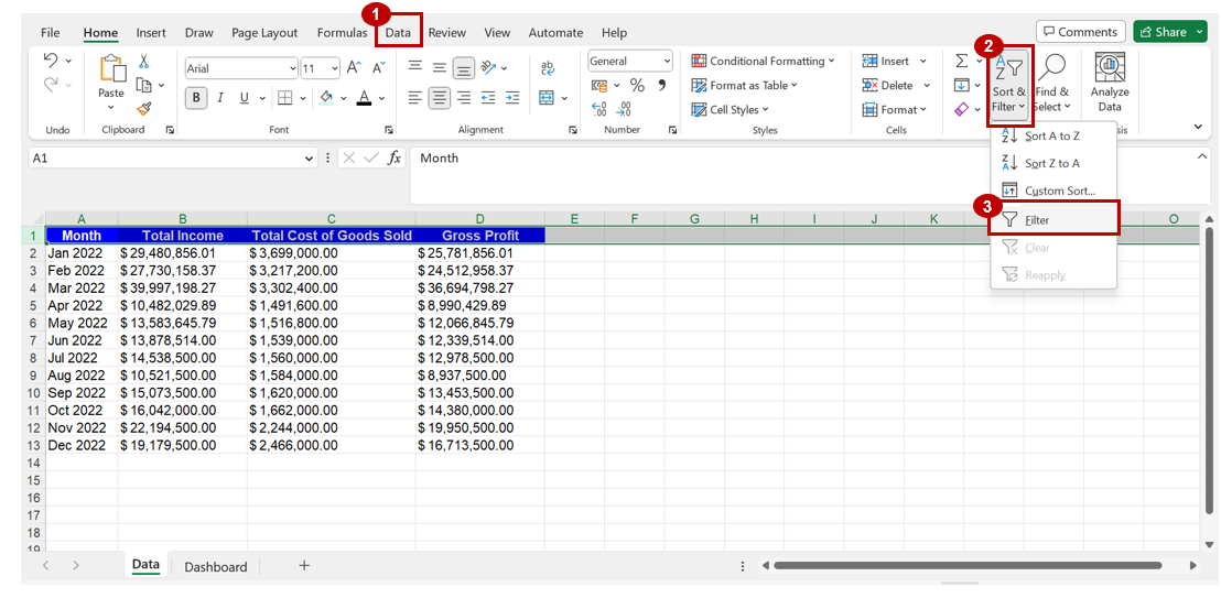
To insert filters in Excel, follow these steps:

1. Click on any cell in the row you wish to apply a filter.
2. Navigate to the ‘Data’ tab in the Excel ribbon.
3. Click on ‘Filter’ in the ‘Sort & Filter’ group. This will apply filter arrows to the row of your cell selected in step 1.

Alternatively, you can press on the “CTRL” (“Command” in case of Mac) + “SHIFT” + “L” keys to add filters.

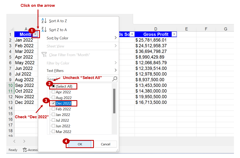
4. Click on the filter arrows to open the filter menu.
5. In the filter menu, the ‘Select All’ option is checked by default. You can uncheck the ‘Select All’ option and then check the boxes next to the values you want to display.
6. Click on “OK” to apply the filter.

For instance: if you want to only display values for the month of December 2022 only, follow the steps displayed in the image below.

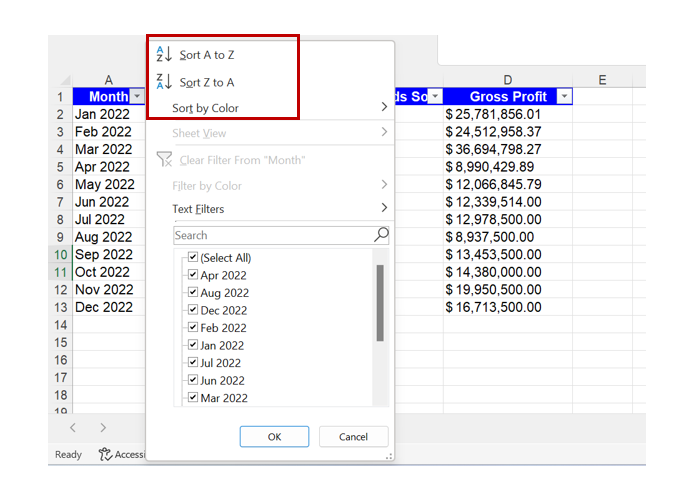
Furthermore, the filter drop-down in excel also allows you to sort by A to Z, sort by Z to A or sort by color.

‍

Basic Filtering: Clearing and Disabling Filters

To clear or disable filters in Excel, follow these steps:

1. Navigate to the ‘Data’ tab in the Excel ribbon.
2. Click on ‘Filter’ again to disable the filter functionality and remove the filter arrows from the header row.

‍

Filtering in Excel is a versatile and powerful feature that allows you to quickly analyze data by displaying only the rows that you wish to see. By mastering basic filtering techniques, you can efficiently sort through large data sets and extract valuable insights. Use this guide to insert filters in Excel and take your data analysis skills to the next level.