DGET Function in Google Sheets: Explained
In this article, you will learn how to use the DGET formula in Google Sheets.
What is the DGET function in Google Sheets?
The DGET function is a database function that basically extracts a single value from a column of a database table or range of cells that meet specified criteria.
You must prepare a well-organized dataset with column headers and a common rule for all database functions, such as DSUM, DCOUNT, and DCOUNTA.
When is the DGET formula beneficial in Google Sheets?
The DGET formula can be helpful in Google Sheets when you need to extract a single value from a database or a range of cells that meet specific criteria. Here are a couple of cases where the DGET formula can be helpful:
- Getting a sales amount from a trade that meets some conditions: For example, if you have a transaction list, you can pick up a sales amount from the database based on customer name, sales region, and sales date.
- Extracting a particular employee ID that satisfies specific requirements: For instance, if you have an employee list that includes name, age, nationality, etc., you can search it for a particular employer ID that meets the criteria you set up.
How to use the DGET function in Google Sheets
You can insert the DGET formula in Google Sheets as follows:
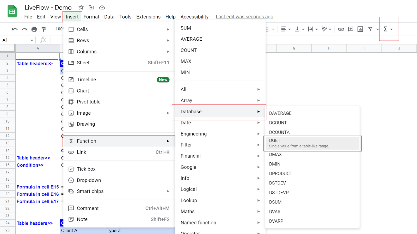
- Type “=DGET(“ or navigate to “Insert” → “Function” (or directly go to the “Functions” icon) → “Database” → “DGET”.
- Select the entire dataset you want to analyze.
- Choose the column header whose number of items you want to compute.
- Input one or more criteria that items should meet.
The general syntax of the DGET formula is as follows:
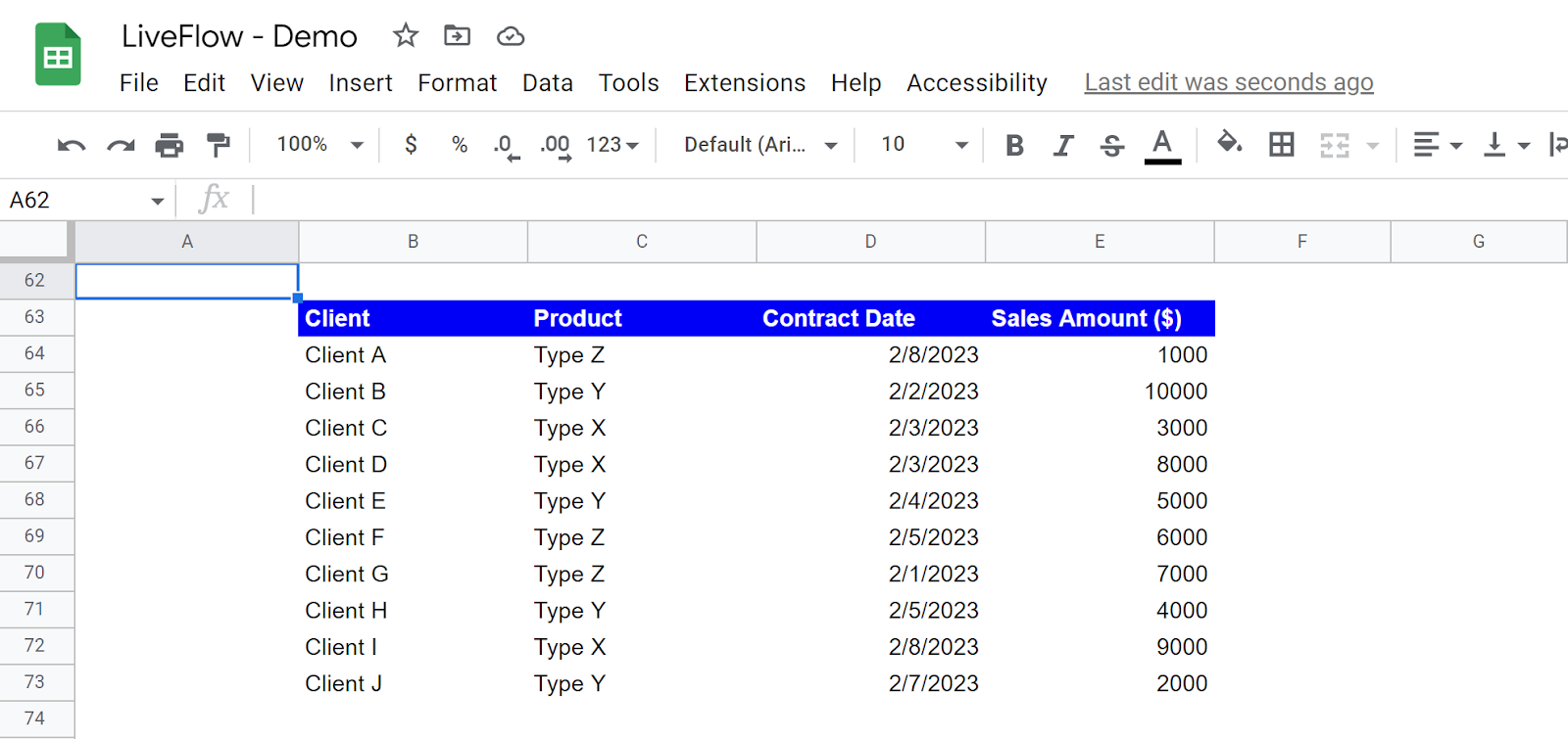
database: This argument should be a range or array whose first row contains table headers (or field names), followed by values in rows (from the second row and downwards) for each field. The “database” could be something like the table in the picture below.
field: This parameter should be one of the column headers in “database”. The formula extracts a value from this column that meets specific condition(s). This argument can be a text string (manual input) of the table header or a column number of the column you want to refer to, assuming the leftmost column in the selected dataset is 1. You can use a cell reference as well.
criteria: This argument should be a range or an array whose first row contains field name(s), followed by specific condition(s) in the second row and downwards.
Note: While the other D-functions aggregate numbers (or the number of items) when you find more than one item that meets specific criteria, the DGET function is the only database function that doesn’t aggregate. Thus, the DGET formula returns an error value to you when it finds more than one match in the dataset. Also. it gives you an error value when it finds no match in the given data
Look at the following cases where we apply the DGET function to the sample sales list above. Imagine you want to know the specific sales amount that meets the criteria you have in mind.
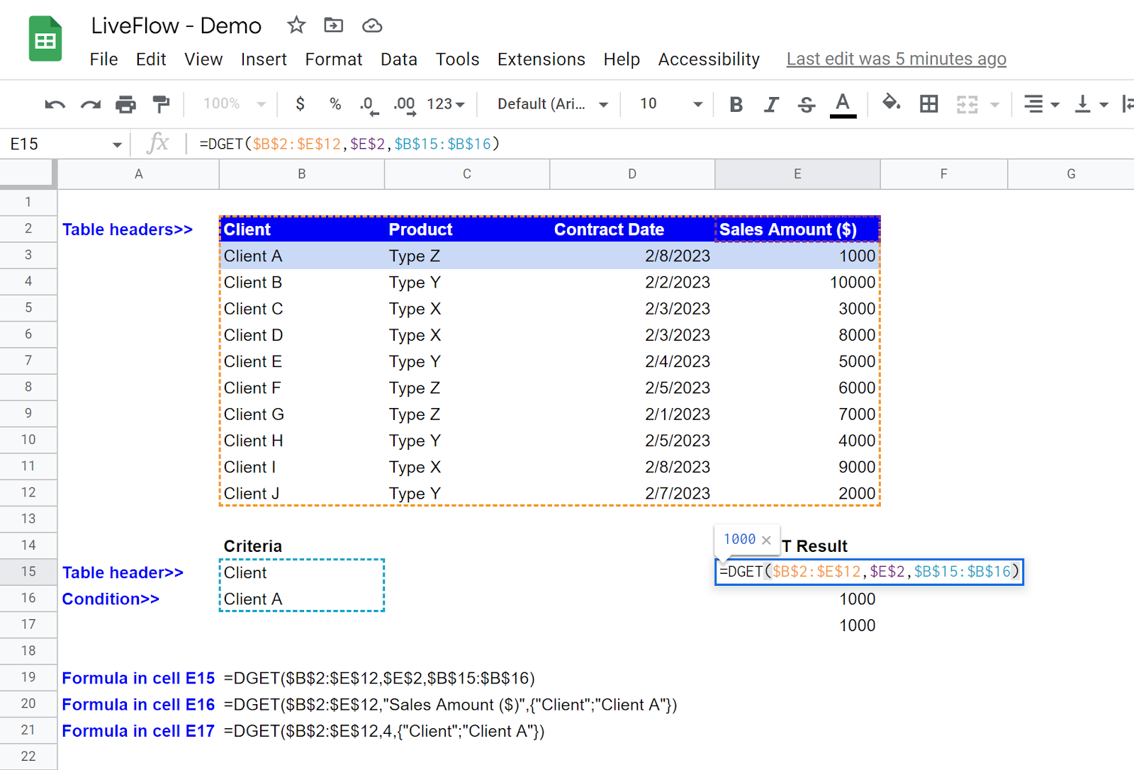
In the first example, assume you need to get the sales from Client A in the list.
- Select the entire table, including the row showing table headers, for the “database” argument.
- Enter the “field” by selecting the cell containing the column header whose column value that meets “criteria” is pulled out.
- Prepare the “criteria” range as shown in the picture below. Enter a table header in a cell and a condition beneath the cell embedding the table header.
- The formula should look as follows.
Although we highly recommend you use cell references in the DGET formula as they make the formula easy to follow and dynamic, if you are keen to use the DGET function with manual inputs for the “field” and “criteria” parameters, you can insert the formula as follow:
Bear in mind that you must enclose text strings with quotation marks and enter a table header and criterion separately, split by a semicolon and surrounded by a pair of curly brackets.
You can replace the table header provided by manual input or cell reference with a column number, 4 in this case, as “Sales Amount” is in the fourth column in the dataset.
With these formulas, you can get the returned value of 1000. The formula extracts 1000 from the first row as the row contains “Client A” in the “Client” column.
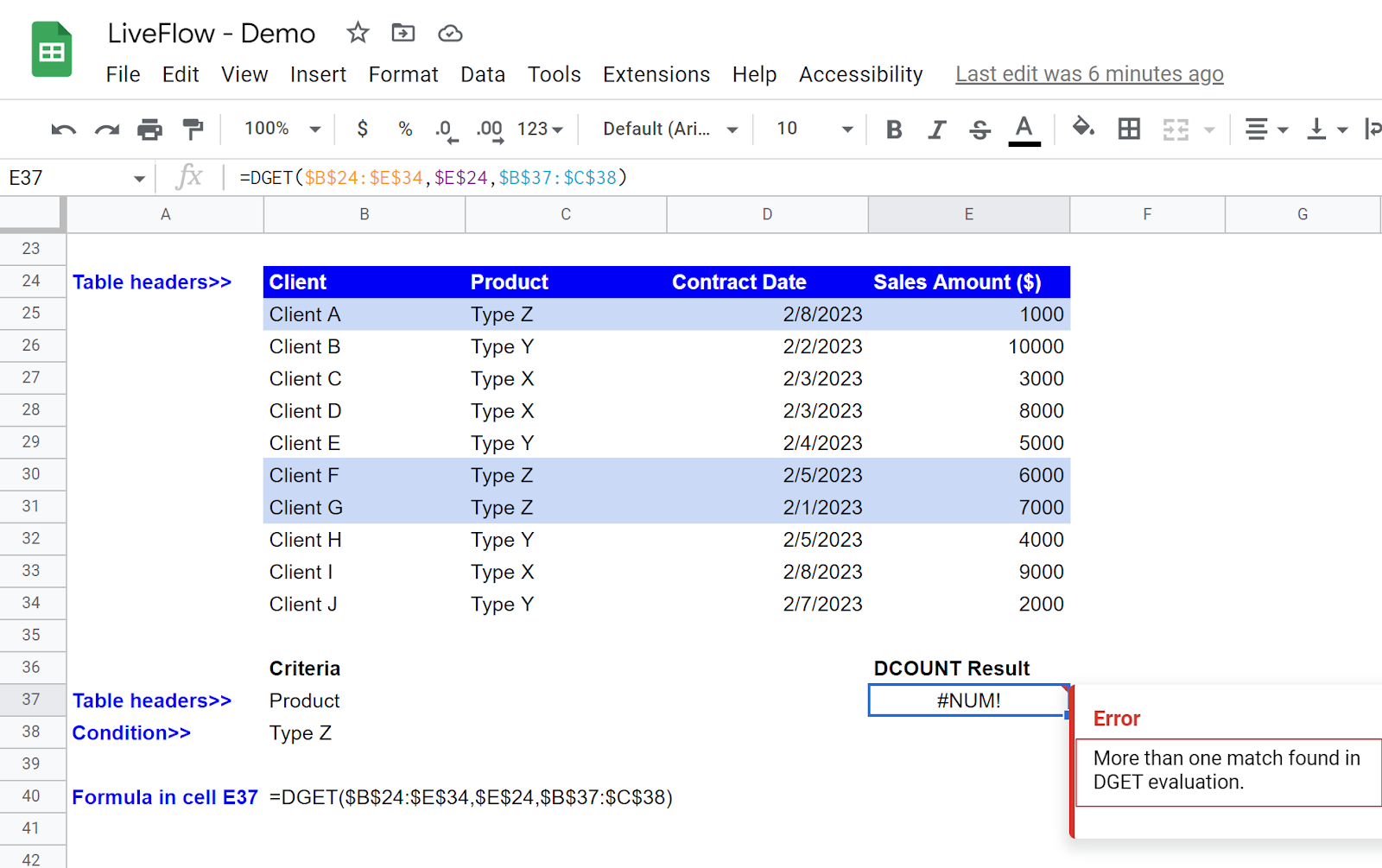
The second example shows when the DGET doesn’t return a proper value. This happens because, as discussed in the note above, the DGET function accepts only one match. As we highlight three rows in the picture, there are three matched if we only consider the “Type Z” product in the sales list.
Thus, the formula can’t identify a match and gives you the “#NUM!# error value.
So, in the third example, consider adding one more criterion that “Contract Date” is “2/5/2023“, in the DGET formula to extract one of the sales values.
As you can see, the formula shows a specific number, 6,000, as only one item meets two requirements. The formulas with cell references and manuals look as follows, respectively:
(Cell reference)
(Manual input)

What are the differences between the DGET and VLOOKUP functions in Google Sheets?
Here are some major differences between the two functions:
- Their general syntaxes look very different, and thus the ways to enter arguments differ.
- Concerning the first point, with the DGET formula, you can extract a specific value from anywhere in the dataset regardless of the order of the columns. However, with the VLOOKUP function, you must locate a column in which the formula finds a match as the most left column in the selected data field and put the column from which the formula pulls out a particular value in the second column or rightwards.
- The DGET formula can extract data based on more than two criteria. In contrast, the VLOOKUP function can only pull out a value that matches a particular lookup value from a specified column, which we could say are equivalent to two conditions.
In summary, the DGET function requires a well-organized dataset with column headings, but it is more flexible in terms of search method and the number of criteria, compared to the VLOOKUP formula.

