
DSUM Function in Google Sheets: Explained
In this article, you will learn how to use the DSUM formula in Google Sheets.
How does the DSUM function work in Google Sheets?
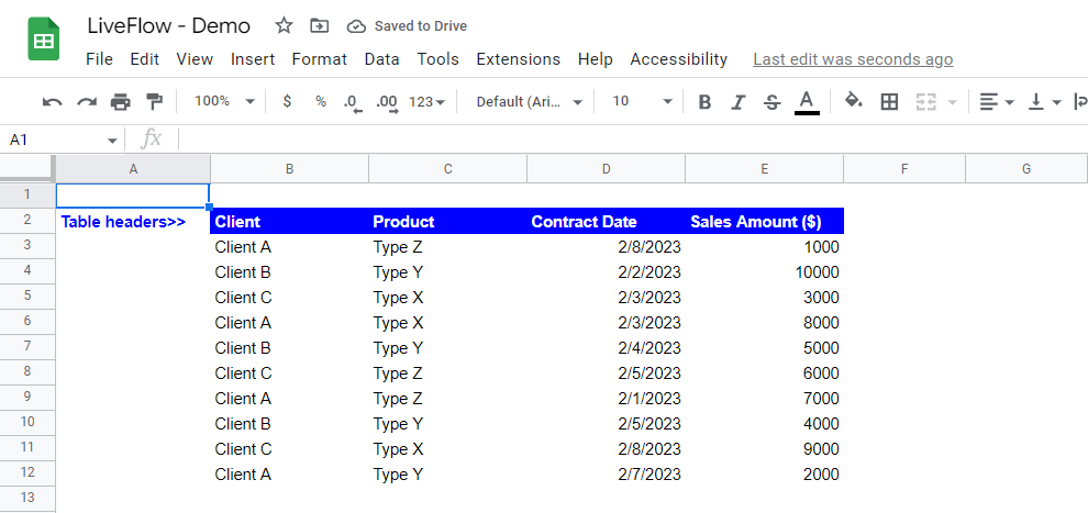
The DSUM function in Google Sheets is similar to the SUMIF or SUMIFS functions. The DSUM calculates the sum of selected database entries based on specific criteria. To use the DSUM formula, you must prepare a dataset with column titles (table headers), such as the sample dataset below.
When is the DSUM formula beneficial in Google Sheets?
The DSUM formula in Google Sheets is beneficial when you need to sum values in a large database or table based on specific criteria. It saves time and effort compared to manually filtering the data and calculating the values, especially when the database is extensive and constantly changing.
Examples of when the DSUM formula can be helpful include:
- Summing sales amounts for a specific product and date range.
- Adding up the expenses for a particular category or account.
- Aggregating the number of units sold for a specific product or SKU.
- Summing the total hours worked for employees in a certain department or role.
How to use the DSUM function in Google Sheets
You can insert the DSUM formula in Google Sheets as follows;
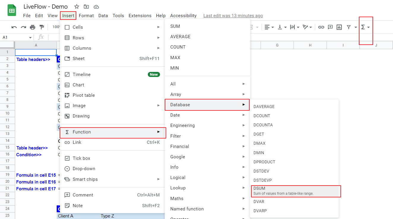
- Type “=DSUM(“ or navigate to “Insert” → “Function” (or directly go to the “Functions” icon) → “Database” → “DSUM”.
- Select the entire dataset you want to analyze.
- Choose the column header whose items you want to sum up.
- Input one or more criteria that items to be added should meet.
The general syntax of the DSUM formula is as follows:
database: This argument should be a range or array whose first row contains table headers (or field names), followed by a value in each row (from the second row and downwards) for each field. The “database” could be something like the table in the picture below.
field: This parameter should be one of the table headers in “database” and the values in this column that meet specific condition(s) are added up by the formula. This argument can be a text string (manual input) of the table header or a column number of the column you want to refer to, assuming the leftmost column in the dataset is 1, or a cell reference containing the text string or column number.
criteria: This argument should be a range or an array whose first row contains field name(s), followed by specific condition(s) in the second row and downwards.
Look at examples in which we apply the DSUM formula to the sample dataset above. Assume you want to calculate the total sales that meet one or more conditions.
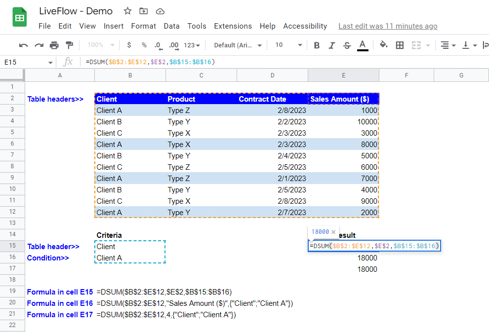
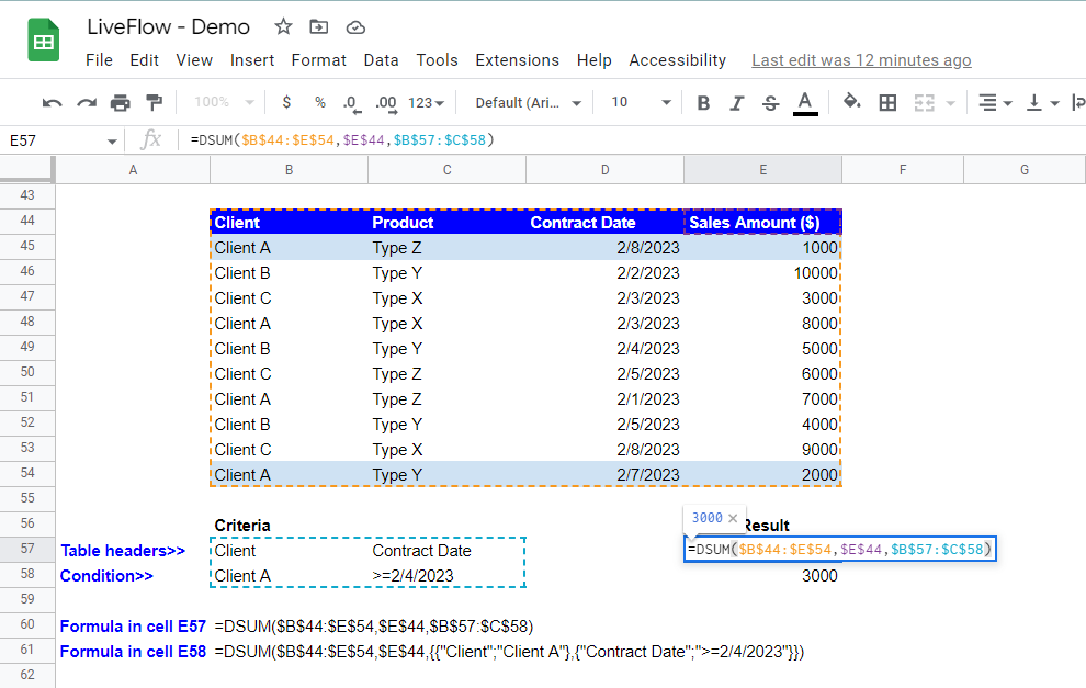
In the first example, imagine you need to calculate the total sales from Client A.
- Select the entire table, including the row showing table headers, for the “database” argument.
- Enter the “field” by selecting the cell containing the column header whose column values that meet “criteria” are aggregated.
- Prepare the “criteria” range as shown in the picture below. Enter a table header in a cell and a condition beneath the cell embedding the table header.
- The formula should look as follows.
Although we strongly recommend you use cell references in the DSUM formula as they make the formula easy to understand and dynamic, if you are interested in using the DSUM function with manual inputs for the “field” and “criteria” parameters, you can insert the formula as follows.
Note that you need to enclose text strings with quotation marks and that you need to enter a table header and a criterion separately, split by a semicolon and enclosed by a pair of curly brackets.
You can replace the table header provided by manual input or cell reference with a column number, 4 in this case, as “Sales Amount” is in the fourth column in the dataset.
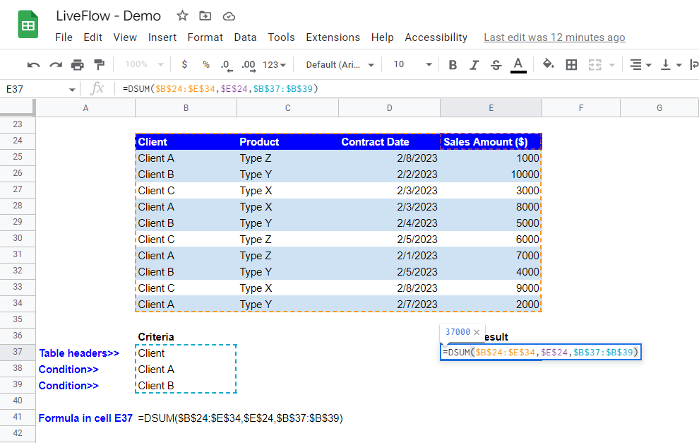
The second example shows the case in which the DSUM formula aggregates the sales when “Client” is “Client A” or “Client B”. Suppose you exclude changes in cell addresses in the DSUM formula. In that case, the only difference between the first and second examples is that a range for the “criteria” is expanded by one cell downwards, as you can see in the following picture.
As you can see, when you want to add one or more conditions for the existing column header used for “criteria”, you enter the additional requirement(s) in the cells right below the first condition. The formula with cell references looks as follows:
The third example presents the case you sum up sales that meet two criteria. Imagine you want to sum up sales contracted with Client A on 2/4/2023 and afterward.
Note that when you add a new table header in “criteria”, you put it in the cell next to the right of the existing table header for “criteria” and enter a specific condition below the cell containing the additional table header. The formula with cell references looks as follows:
(The formula with manual inputs)
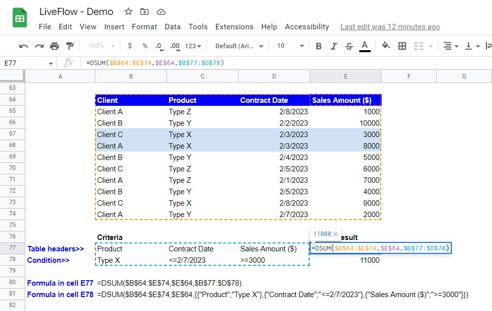
The last example shows the DSUM function containing three requirements. Assume that you need to add up sales that meet three conditions: (i) “Product” is “Type X”, (ii) “Contract Date” is on or before 2/7/2023, and (iii) “Sale Amount ($)” is equal to or greater than 3000. You can create the formula with cell references as follows:
For the formula with manual inputs, you must (i) enclose each pair of a table header, and a specific criterion with curly brackets, (ii) divide each chunk enclosed by the curly brackets by a comma, and (iii) enclose all chunks separated by a comma with a pair of curly brackets.
What is the difference between the DSUM and SUMIFS?
The DSUM and SUMIFS functions in Google Sheets sum up values in a database or table based on specific criteria and return the same results if their arguments are input properly, but they have some differences:
- Dataset: To use the DSUM function, you need to organize your dataset so that each column in the data table has each table header representing values in the column, as all arguments required need these table headers as input (or a part of the input). On the other hand, when you use the SUMIFS function, you don’t necessarily make a well-organized data table with column titles (though it is highly recommended).
- Criteria: You need to include all conditions in a range or an array as it accepts only one argument for “criteria” in the DSUM formula, but in the SUMIFS formula, you need to incorporate pairs of criteria and the ranges for the criteria until you include all conditions. So, if the data volume is much larger, the DSUM formula can work more efficiently than the SUMIFS function.


