ISNA Function in Excel: Explained

In this article, you will learn what is the ISNA formula in Excel and how to use it.

‍

What is the ISNA formula in Excel?

The ISNA formula in Excel is used to check whether a specific value or a formula result returns the #N/A error. The #N/A error indicates that the value being looked up or referenced is not available or not found. It returns TRUE or FALSE as the output.

‍

Uses of ISNA formula in Excel

The ISNA function in Excel is mainly used for error handling and data validation purposes. Some of the most common uses of the ISNA function are:

1. Checking for #N/A errors: You can use the function to identify cells with #N/A errors and take appropriate action, such as replacing the error with a value or modifying the formula to avoid the error.
2. Nested formulas: The ISNA function can be used in combination with other functions, such as IF and IFERROR, to create more complex formulas. For example, you can use the function to test whether a VLOOKUP or INDEX formula returns an #N/A error, and then return a specific value or message if it does.
3. Data validation: The ISNA function can be used in data validation rules to ensure that users enter valid data. For example, you can set up a validation rule that requires users to enter a value that is not equal to #N/A in a specific cell or range.

‍

How to use the ISNA formula in Excel

Syntax: 

=ISNA(value)

Where, value - is the cell or range of cells you want to check.

1. Select the cell where you want to display the outcome.
2. Type the following formula into the cell: =ISNA(
3. Enter the value after the open parenthesis and then close the parenthesis.

‍

Sample use case for ISNA function in Excel

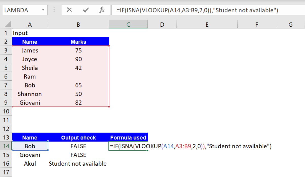
Suppose you have a list of students with their scores in a particular paper and you want to cross-check against a separate list which of the students did not appear for the exam. 

‍

You can use a combination of IF, VLOOKUP, and ISNA to accomplish this:

Step 1: Enter the names of student you want to check starting Cell A14

Step 2: Enter the following formula in the column next to it (B14):

=IF(ISNA(VLOOKUP(A14,A3:B9,2,0)),"Student not available")

Step 3: Drag the formula down for all the cells

Step 4: Refresh the formulas to see the results.

‍

If the student is a part of the original list with grades you should see ‘FALSE’ as the output. This is because the function of ISNA is to return either TRUE or FALSE depending on the condition being satisfied.

‍

‍