
How to Use IFERROR Formula in Excel: Quick How-To Guide
Errors in Excel can be frustrating and potentially lead to confusion or misinterpretation of data. By using the IFERROR function, you can manage these errors in a more efficient and user-friendly manner. This how-to guide will explain the essentials of the IFERROR formula in Excel, detailing its uses, syntax, and how to insert it into your spreadsheet. By the end of this guide, you'll have a solid understanding of the IFERROR function and how it can help you create cleaner, more reliable worksheets.
What is the IFERROR function in Excel used for?
The IFERROR function in Excel is designed to handle and manage errors that may arise in formulas, such as ‘#DIV/0!’, ‘#VALUE!’, or ‘#N/A’. It allows you to specify an alternative value or action to be taken when an error occurs in Excel, making your worksheets more informative and visually appealing. With the IFERROR formula, you can replace error messages with a custom message, a blank cell, or an alternative calculation.
Understanding the IFERROR formula syntax in Excel
The syntax for the IFERROR function in Excel is as follows:
- value: The formula or expression you want to evaluate for errors (e.g., a division operation or a VLOOKUP formula).
- value_if_error: The value to be returned if the value parameter results in an error (e.g., a custom message, a blank cell, or an alternative calculation).
When to use the IFERROR function in Excel
The IFERROR function in Excel is particularly useful when:
- Managing complex Excel worksheets with multiple formulas that may generate errors.
- Presenting data to others in a visually appealing and easy-to-understand manner.
- Simplifying troubleshooting by identifying formulas that may be causing errors and replacing them with more informative messages.
Inserting the IFERROR formula in Excel
To insert the IFERROR formula into your Excel spreadsheet, follow these steps:
Step 1: Identify the cell where you want to display the result of the formula.
Step 2: Click on the selected cell and start typing the formula “=IFERROR” and click on the formula prompt that opens up.
Replace ‘value’ with the formula or cell you want to evaluate for errors, and ‘value_if_error’ with the value or action to be taken if an error occurs.
Step 3: Press the “ENTER” key to complete the formula.
Excel will now evaluate the formula and display the specified ‘value_if_error’ if an error is encountered, or the result of the value parameter if no error occurs.
Use case of the IFERROR function in Excel
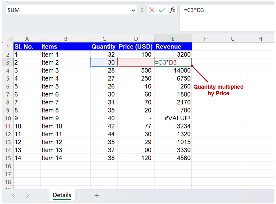
In the below example, the quantity multiplied by the price for item 2 will return a ‘#VALUE!’ error since the price for item 2 is not saved in the price catalog. The same is the case with item 9, as displayed in the image below.
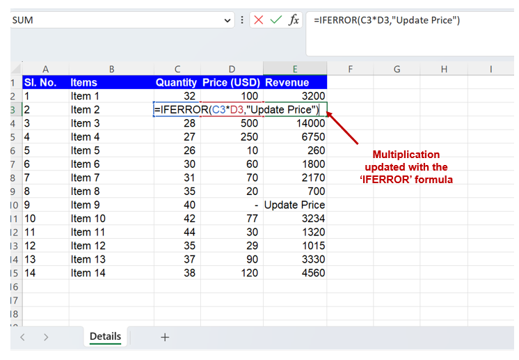
If the same formula is updated with the IFERROR formula, where ‘value’ is quantity * price and ‘value_if_error’ is updated to “Update Price” or any other free-form text, the missing price for items 2 and item 9 can be easily identified and rectified.
Conclusion:
The IFERROR function in Excel is a powerful tool for managing and handling errors in your worksheets, allowing you to create cleaner, more user-friendly spreadsheets. By understanding the syntax and use cases of the IFERROR formula, you can enhance your Excel skills and improve the reliability of your data.