LEFT Function in Excel: Explained

In this article, you will learn how to use the LEFT formula in Excel.

‍

What is the LEFT formula in Excel?

The LEFT formula in Excel extracts a specified number of characters from the beginning of a text string. 

‍

When is the LEFT function useful in Excel?

The LEFT function in Excel is beneficial when you want to extract a specific portion of a text string. For example, you might use it to pull out the prefix of an ID number. It is also useful when extracting the first few characters of a text string to sort or filter the data. For example, you might use the LEFT function to extract the first letter of each word in a list of names to group them alphabetically. It can also be combined with other functions, such as the CONCATENATE function, to extract a specific portion of a text string and then combine it with another text string.

‍

How to use the LEFT formula in Excel

The general syntax for the formula is as follows: 

=LEFT(text, [num_chars]) 

The "text" argument is the text string you want to extract characters from, and the "num_chars" argument is the number of characters you want to extract, starting from the left. The formula will return the entire text string if the "num_chars" argument is omitted.

‍Note: The “num_chars” parameter must be equal to or larger than zero. When “num_chars” is larger than the length of a text string, the LEFT function returns the entire text string. If the “num_chars” argument is left blank, the formula considers that it is 1.

‍

Look at the following examples to understand the LEFT function better.

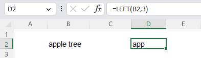
Example:

=LEFT(B2,3)

In this example, B2 contains "apple tree," and the formula would return "app".

‍

You can also use the LEFT function in a more complex formula, such as combining it with other functions, like CONCATENATE, to extract a specific portion of a text string and then combine it with another text string.

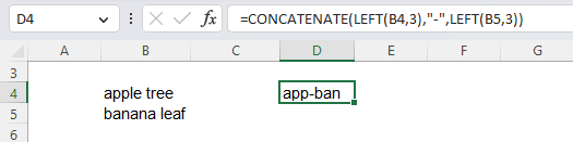
An example formula is as follows::

=CONCATENATE(LEFT(B4,3),"-",LEFT(B5,3)) 

In this case, B4 contains "apple tree", and B5 contains "banana leaf". The formula would return "app-ban", as shown below in the picture.

‍

Finally, note that the LEFT function is case-sensitive, as shown in the screenshot below. So, “liveflow” and “LiveFlow” are considered different by the LEFT function.

‍

Analyze your live financial data in a snap in Google Sheets

Are you learning this formula to visualize financial data, build a financial model, or conduct financial analysis? In that case, LiveFlow may help you automate manual workflows, update numbers in real-time, and save time. You can access various financial templates on our website, from the simple Income Statement to Multi-Currency Consolidated Financial Statement. Are you interested in this product but are an Excel user? That’s not a problem at all. You can connect Google Sheets to Excel quickly. 

To learn more about LiveFlow, book a demo.