
SUMIFS Function in Google Sheets: Explained
In this article, you will learn how to use the SUMIFS formula in Google Sheets.
What is the SUMIFS function in Google Sheets?
The SUMIFS function in Google Sheets is used to sum the values in a range that meets multiple criteria.
When is the SUMIFS formula helpful in Google Sheets?
The SUMIFS formula is beneficial in Google Sheets when you need to add the values in a range based on various requirements and find specific information quickly.
For example, if you have a large sales data dataset and want to see the total sales for a particular product and region, you can use the SUMIFS function to sum the values in the sales column that meet both of those criteria.
Another example is that if you have a sheet that tracks expenses and want to find the total amount spent on a specific category of payments in a particular month, you can use the SUMIFS function to sum the values in the expense column that meet both of these criteria.
How to use the SUMIFS formula in Google Sheets
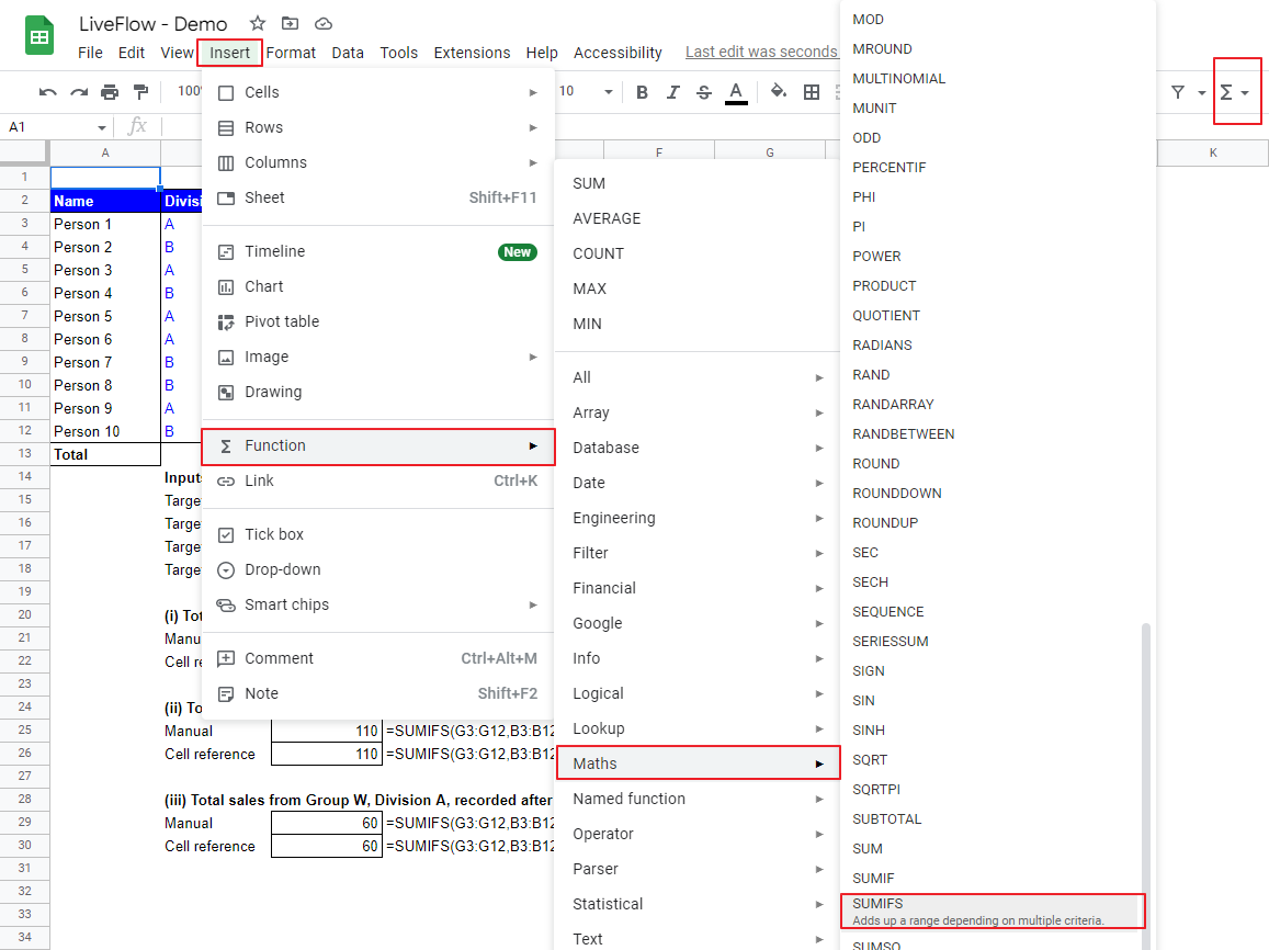
- In a chosen cell, type “=SUMIFS(” or select it from a list of functions (Go to the “Insert” tab, ➝ “Function” ➝ “Maths” ➝“SUMIFS” function).
- Select a range to be summed up and enter all criteria and ranges for them.
- Press the “Enter” key on your keyboard.
The following is a generic formula of the SUMIFS function.
sum_range: This is a range that you want to add up
criteria_range 1: This is a range where you want to check if each cell in this range matches a criterion
criterion 1: This is a specific condition you would like to apply to the selected range (Criteria_range 1).
criteria_range 2 [Optional]: When you add other standards, you also need to specify the ranges for the additional requirements.
criteria 2 [Optional]: You can include other requirements, if any.
You will need to repeat inputting a pair of a criterion and a range until you incorporate all conditions.
Note: The number of cells in the selected ranges should be equal. The SUMIFS shows a total number that meets all criteria input.
Let’s see examples of how the function works with the following dataset. Imagine you want to understand your company’s sales performance by division from different standpoints.
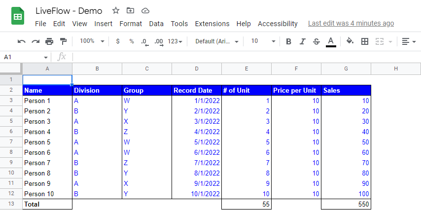
In the examples, you will find two types of inputs in the formulas, manual input and cell reference. The manual input means you type criteria manually and directly in the formulas, and the cell reference means that you refer to particular cell(s) containing a specific number, date, or text.
We highly recommend you take the latter approach as it is more flexible and helps you reduce mistakes, such as leaving an old criterion when you change the formula.

Total Sales from Group W, Division A
In the first example, the criteria are two inputs, “Division” and “Group”.
The “Inputs” group of cells defines our targets such as Group and Division.
The formula in cells C21 and C22 calculates how many sales Group W from Division A made in total and gives us the result we’re looking for.
Total Sales from Group W, Division A, recorded after 4/30/2022
The second example adds one more criterion, “Recorded Date”, so the outcome is the sales for Group W, Division A, recorded after 4/30/2022. You can see the values returned by the SUMIFS formulas in cells C25 and C26.
Total Sales from Group W, Division A, recorded after 4/30/2022, with the number of units greater than or equal to 6
In the third example, the number of units - “# of Unit” - is also included on top of the existing three criteria. The returned values are shown in cells C29 and C30.
Regardless of the approach you take, bear the following rules in mind:
- Numbers and cell references are not needed to be input with quotation marks.
- Text, wildcard (signs such as “*,” “?,” and “~.”), and date need to be enclosed with quotation marks, such as “A” or “*” or “8/25/2022”.
- Comparison operators such as “=,” “<,” and “>” with figures, text, and dates need to be enclosed by double quotes such as “<=100,” “<>apple,” and “>8/25/2022”.
- Comparison operator(s) with cell reference(s) or another formula(s) should require (i) quotation marks to enclose them, and (ii) “&” (ampersand) between the operators and formula(s) like “>=”&A1 or “<”&TODAY().
How do I SUMIFS multiple criteria in one column in Google Sheets?
For simplification, let’s assume the number of criteria is two.
When you want to incorporate more than one criteria in a column, you can use curly brackets “{}” and the SUMIFS formula looks like this; =SUMIFS(sum_range W, criteria_range X, {criterion Y, criterion Z}). This formula brings you the total value of cells that match the criteria of C or D.
Here is another way to do this, but this approach is a bit more burdensome as you need to use SUMIFS functions as many as the criteria. Again, let’s assume you want to apply two standards to a column.
You need to add up two results of SUMIFS functions, and it should look like this; =SUMIFS(sum_range A, criteria_range B, criterion C)+SUMIFS(sum_range A, criteria_range B, criterion D); or you can use two SUMIF functions as well, and it should look like this; =SUMIF(range B, criterion C, [sum_range A])+SUMIF(range B, criterion D, [sum_range A]).
What is the difference between SUMIF and SUMIFS?
The SUMIF formula shows the total figures in cells which match a condition. The SUMIFS function gives you the total figures in cells which meet multiple criteria. As you can see above, you can use both formulas, if you consider only one condition.
However, you should be aware that the order of mandatory inputs in the two functions is different. Also, if you want to consider multiple conditions, it is better to use the SUMIFS function instead of the SUMIF formula. Move on to How to Use SUMIF formula in Google Sheets to learn the SUMIF function.


