
DETECTLANGUAGE Function in Google Sheets: Explained
In this article, you will learn how to use the DETECTLANGUAGE formula in Google Sheets.
What does the DETECTLANGUAGE formula do in Google Sheets?
The DETECTLANGUAGE function in Google Sheets detects the language of a given text string. It returns the language code for the detected language. For example, if you use the formula =DETECTLANGUAGE("Bonjour"), it will return fr, indicating that the text is written in French.
The DETECTLANGUAGE formula is helpful for cases where you have a spreadsheet with text in multiple languages and want to identify each cell's language. You can then use this information to perform language-specific operations on the text, such as using a translation formula to translate the text into another language.
Keep in mind that the DETECTLANGUAGE formula is not always accurate, and it may not be able to detect the language of some text strings. It is also important to note that the formula is only available in Google Sheets and not in other spreadsheet programs such as Microsoft Excel.
How to use the DETECTLANGUAGE function in Google Sheets?
Here is the syntax for the DETECTLANGUAGE formula:
Text_or_range: The text for which you want to detect the language. This can be a cell reference or a string value manually input. Don’t forget to enclose the manual text input with quotation marks.
Note: If the selected range includes multiple languages, the first text found will be evaluated, and the formula returns the language code for the first text string.
For example, if you use the formula below,
it will return “fr”, indicating that the text is written in French.
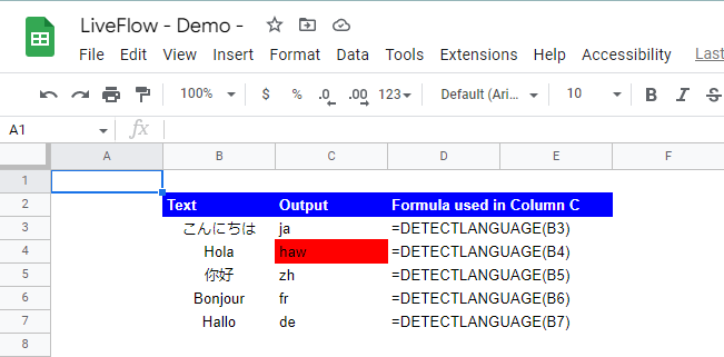
Here are examples of how the DETECTLANGUAGE formula works with a cell reference input in Google Sheets. Note that, as touched upon in the section above, the DETECTLANGUAGE function is not perfect. As you can see in the picture, the function considers “hola” a language different from Spanish.
You can use the detected language code to translate the text to another language using the GOOGLETRANSLATE function in Google Sheets. Check the article below if you want to learn how to use the GOOGLETRANSLATE formula in Google Sheets.
GOOGLETRANSLATE Function in Google Sheets: Explained


