
How to Use MATCH Function in Google Sheets
In this article, you will learn how to use the MATCH formula in Google Sheets. This function is beneficial when you want to know a relative position of an item in a specific range.
How to use the MATCH formula in Google Sheets
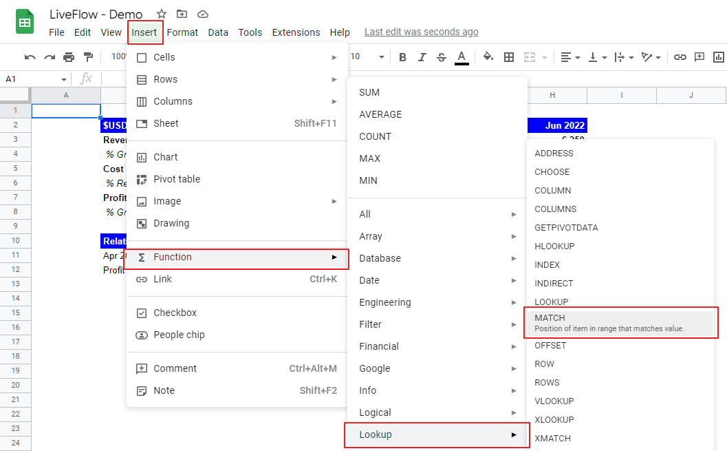
- Type “=MATCH” or go to “Insert” → “Function” → “Lookup” → “MATCH”.
- Input a “search_key” by manual input or cell reference
- Select a range in which you will find a match with the “search_key”.
- Define how to search if necessary.
The generic formula is as follows:
This function is useful if you want to find a relative position of an item in a particular range.
Search_key: This is a value whose relative position you want to find in a range
Range: This is a range in which you want to know the relative position of the “search_key” This range should be one-dimensional - a row or a column.
[search_type]: This is the optional input. You can input 1, 0, or -1. If you enter nothing, the formula assumes 1 is entered. Each number has the following effect on the formula’s search.
1: If you enter “1”, the formula looks for the largest value less than or equal to the “search_key” when the range is sorted in ascending order.
0: This is for an exact match. You can use this when the data set is unsorted.
-1: With this number, the formula tries to find the lowest value larger than or equal to the “search_key” when the range is sorted in descending order.
Imagine you are a finance manager and want to know the relative locations of specific items, “Apr 2022” and “Profit” in the data set in the picture below. More specifically, you need to know which column the data for “Apr 2022” is and which row the “Profit” data is.
The relative location of “Apr 2022” in the selected range
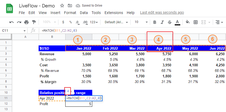
The assumptions in the formula in the picture above are as follows:
Search_key: B11 (“Apr 2022”)
Range: C2:H2 (a row)
[search_type]: 0 - an exact match
The formula returns 4 because “Apr 2022” is in the fourth column in the selected range. Note that the function does not give the Google Sheets’ row index.
The relative position of “Profit” in the chosen array
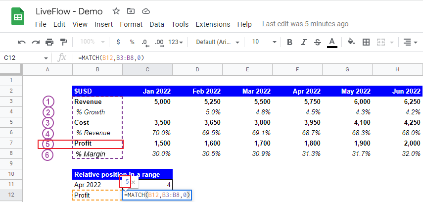
The assumptions in the function in the screenshot above are as follows:
Search_key: B12 (“Profit”)
Range: B3:B8 (a column)
[search_type]: 0 - an exact match
The formula returns 5 because “Profit” is in the fifth row in the selected range. Note that the function does not give the Google Sheets’ column index, either.
Why is the MATCH formula not working?
- No exact match: There is no exact match when you input 0 for “search_type” in the formula. Extra spaces contained in “search_type” or a target value don’t allow the exact match to work properly.
- Incorrect range selection: You choose the wrong range for search in the formula
- Format difference: The format of value whose relative position you are trying to find is different from that of a “search_key”
- Unsorted data: When you choose “1” or “-1” for “search_type”, the range you select should be sorted as a chosen search method assumes - in ascending order for 1, and in descending order for “-1”
How do I use INDEX/MATCH in Google Sheets?
Check this article to learn what INDEX/MATCH is and how to use it in a practical situation.
What is the alternative to the MATCH function?
One of its alternatives is the XMATCH function. The formula provides the same search function with more flexible search methods.
How do I match the same data in Google Sheets?
One of the ways to find the same data is to use Conditional Formatting. Check this article to learn how to highlight duplicates in a data set.