
How to Highlight Duplicates in Google Sheets
In this article, you will learn how to highlight duplicates with Conditional Formatting in Google Sheets.
How to use Conditional Formatting to highlight duplicates in Google Sheets
- Select a range or array you want to find and highlight the duplicates.
- Go to the “Format”→ “Conditional formatting”.
- Choose a range to which you apply Conditional Formatting.
- Select “Custom formula is” and enter the COUNTIF formula such as “=COUNTIF(range, tested value)>1”.
- Click “Done” at the bottom right.
Assume you look at some survey data and want to check if there are any duplications in the data.
First, look at the example below where you highlight the duplications in the Name column.
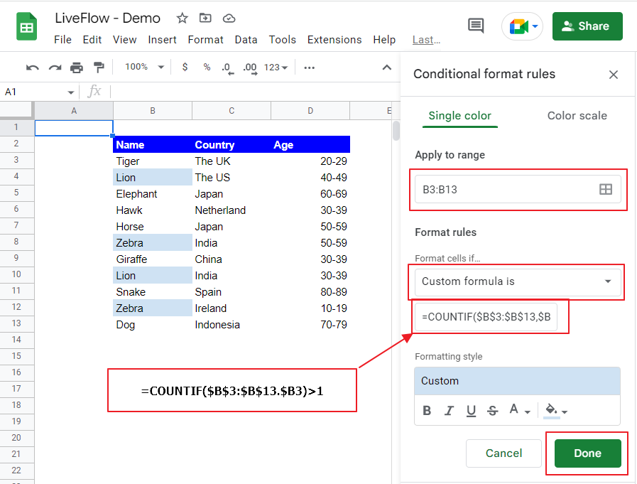
The range should be data in the Name column, B3:B13, as you are looking for duplicates there. You use the COUNTIF formula to test each cell value from B3 to B13, such as “Tiger” and “Lion” and see how many values match the tested value in the selected range. If there is any duplication for a tested word, the COUNTIF formula returns “2” or above.
So, the “Format cells if…” section defined that if the number given by the COUNTIF for a tested cell is more than 1, the cell should be highlighted. As such, the range should be the absolute reference, whereas a tested cell should be the partial absolute reference. [Insert a link to an article about reference]
How do I find duplicates in multiple columns in Google Sheets?
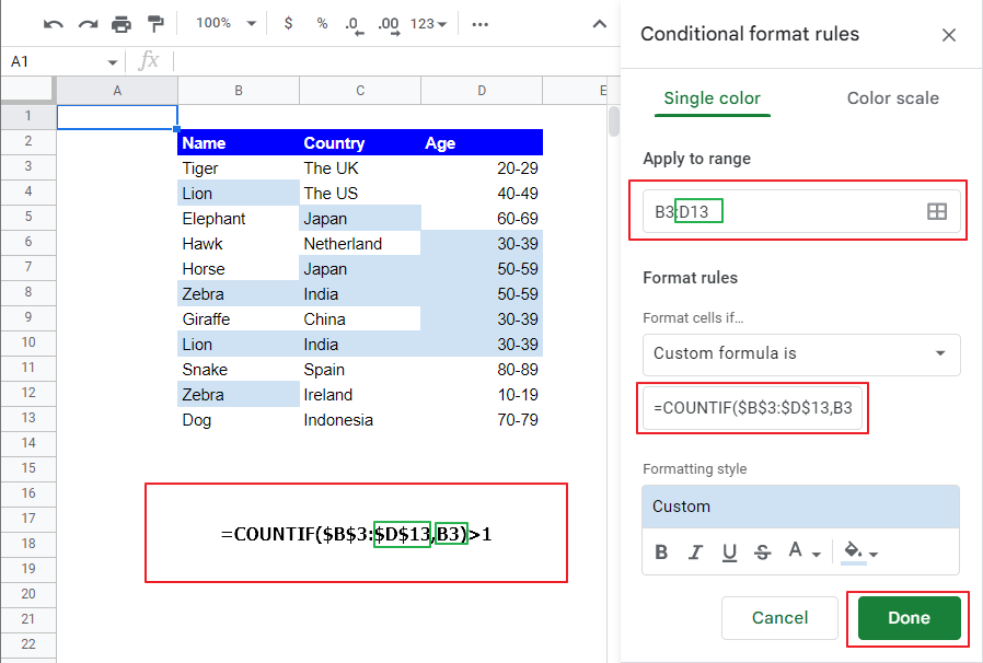
If you want to spotlight duplicates across multiple columns, you need to tweak the range and the COUNTIF function, as shown below.
There are three major changes:
(i) The range for the Conditional Formatting should be the entire list - B3:D13
(ii) The range for the COUNTIF function should be the entire list as well
(iii) The tested value in the COUNTIF function should be a relative reference, not a partial absolute reference because you need to test all values in the list.
If you want to highlight these duplicated values in different colors, you need to set up the Conditional Formatting rules - in this case, three rules - by columns and select different fill colors for each rule.
Check this article [A hyperlink to be inserted] if you are keen to learn how to use Conditional Formatting based on another cell value first.


