TEXT Function in Google Sheets: Explained

In this article, you will learn how to use the TEXT formula in Google Sheets. This function is beneficial when you insert narratives, such as ones about a financial statement or a KPI dashboard, by combining cell references and manual input.

‍

How to use the TEXT function in Google Sheets

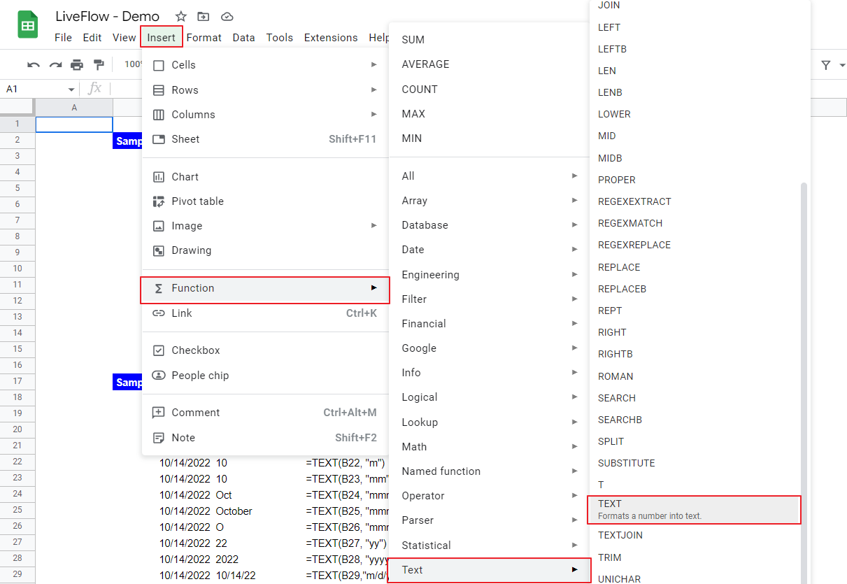
1. Type “=TEXT” or navigate to the “Insert” tab (or “Functions” icon) → “Function” → “TEXT” → “TEXT”.
2. Input a value whose formatting you want to change by manual input or cell reference.
3. Define the formatting and insert the argument accordingly.
4. Press the “Enter” key.

‍

The general syntax is as follows:

=TEXT(number, format)

Number: This is a value, such as a number, date, or time, whose formatting you want to change

Format: The formatting you want to apply to the “number”. There are two patterns for this argument: "0” and “#” or date and time format. You can't mix them. Also, don’t forget to enclose the inserted format with quotation marks.

‍

Notes

1. You can’t enter “*”, an asterisk mark, or “?”, a question mark in the “format” argument.
2. The TEXT formula can’t show a fractional pattern.

‍

“0” and “#” formatting

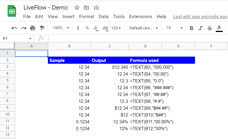
0: If you input 0,  when a number to be formatted has fewer digits than the number of “0” in the argument, 0 is forcefully shown. For instance, =TEXT(12.34, “000.000”) returns 012.340. On the other hand, if a number to be converted has more digits to the right of the decimal point than the defined formatting, they are rounded at the place equivalent to the number of zeros (to the right of the decimal point). For example, =TEXT(12.34, “0.0”) returns 12.3.

#: This sign works similarly to 0. However, it doesn’t display zeros on either side of the decimal point. For instance, =TEXT(12.34, “###.###”) shows 12.34.

‍

Date and time formatting

In this format, some alphabets are assigned to specific items (e.g., d for date and day of the week, m for month, and y for year). The number of a particular alphabet defines the detailed format. Look at the descriptions below.

‍

Date/Day

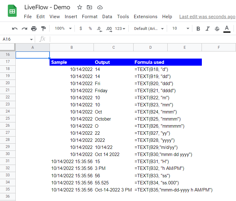
d: the day of the month as one or two digits.

dd: the day of the month as two digits.

ddd: the short name of the day of the week.

dddd: the full name of the day of the week.

‍

Month

m: the month of the year as one or two digits or the number of minutes in a time (e.g., 4). This letter represents month unless it is used with other alphabets such as “h” and “s” to show time.

mm: the month of the year as two digits or the number of minutes in a time. If the original month is single digit, then zero is added to the left (e.g., 04). Again, this letter represents month unless it is used with other alphabets such as “h” and “s” to show time.

mmm: the short name of the month of the year (e.g., Apr).

mmmm: the full name of the month of the year (e.g., April).

mmmmm: the first letter in the month of the year (e.g., A).

‍

Year

yy: the year as two digits (e.g., 22).

yyyy: for the year as four digits (e.g., 2022).

‍

Hour

H/HH: the hour on a 24-hour clock (e.g.,14 for 2PM).

h/hh: for the hour on a 12-hour clock (e.g., 2 for 2PM).

Note: The effect of the number of letters is the same as the one for “m/mm”.

‍

Minute

m/mm: for the number of minutes (e.g., 32)

‍

ss: for the seconds in a time.

ss.000: for milliseconds in a time.

‍

AM/PM: showing “AM” or “PM” according to the time of day.

‍

Here is an example of a template that allows you to have the latest financial and thus updated narratives in Google Sheets: Turn Reports Into Simple Narratives Template - Google Sheets & Excel