How to Remove #DIV/0! in Google Sheets
A #DIV/0! Error in Google Sheets can be frustrating and unpleasant to look at in your spreadsheet.
This article will explain how to get rid of the unsightly return value in your sheet.
What Causes a #DIV/0 Error?
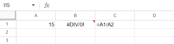
A #DIV/0 error occurs when you are attempting to run a formula and either have a complete lack of a denominator or your denominator is 0 when dividing.
You cannot divide any number by 0 so this returns an error and does not allow you to run your formula for the given cell.
Luckily we do not have to look at the error message by just following a few simple steps.
How to Get Rid of #DIV/0 Error
Thankfully, Google Sheets has a built in fix that allows you to display your text of choice when an error occurs. For this fix, we will be using the IFERROR function.
The IFERROR function syntax is as follows:
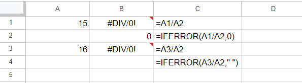
Value: This will be where you perform your math. This is where you will type exactly what is shown in cell C1 in the example above.
Value_if_error: This is where you will select what is to be displayed if an error occurs. In our example, we will show how to make this both a 0 and a blank cell.
IFERROR With a 0 Displayed
First, we will go over how to display a 0 in the cell that has the #DIV/0! Error. To do this, our IFERROR function will be utilized by typing “IFERROR(“ into our cell. Following the syntax of the formula, we will first fill in the ‘value’ for our IFERROR.
Assuming the same setup as our example from the picture above, our value will remain the same: A1/A2. The next step is to choose what will be displayed if an error occurs.
Since we are choosing to display a number, we just type a 0 in the second argument of our function and press enter. It should look something like the example below.
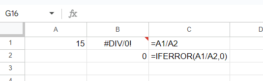
The exact same division was run in cells B1 and B2, B2 just has a more aesthetically pleasing appearance due to our IFERROR function. Next, we will go over how to display a blank cell rather than showing an error or a 0.
IFERROR with a Blank Cell Displayed
In order to get our formula to return a blank cell in case of error, we will follow the same steps as above with a small tweak at the end.
Once again, we will be utilizing the IFERROR function. Once we have completed the first argument as we did above, we will need to type a blank into the ‘value_if_error’ portion of the formula. To do this, we need to type quotes with a blank space in the middle.
It will look like this “ “ inside your formula. An example of this in Google Sheets is shown below. Note cell B4 has a formula run on it.