SEARCH Function in Google Sheets: Explained

In this article, you will learn how to use the SEARCH formula in Google Sheets. The SEARCH formula returns an integer to show a position at which a particular string is found first in a specific text. Thus, the SEARCH function is beneficial when finding a particular word's location or a combination of letters in text strings. You can leverage this function even when you only need to know whether a word is contained in a text. Note this function is not case-sensitive. If you need a case-sensitive search, use the FIND formula instead.

‍

How to use the SEARCH function in Google Sheets

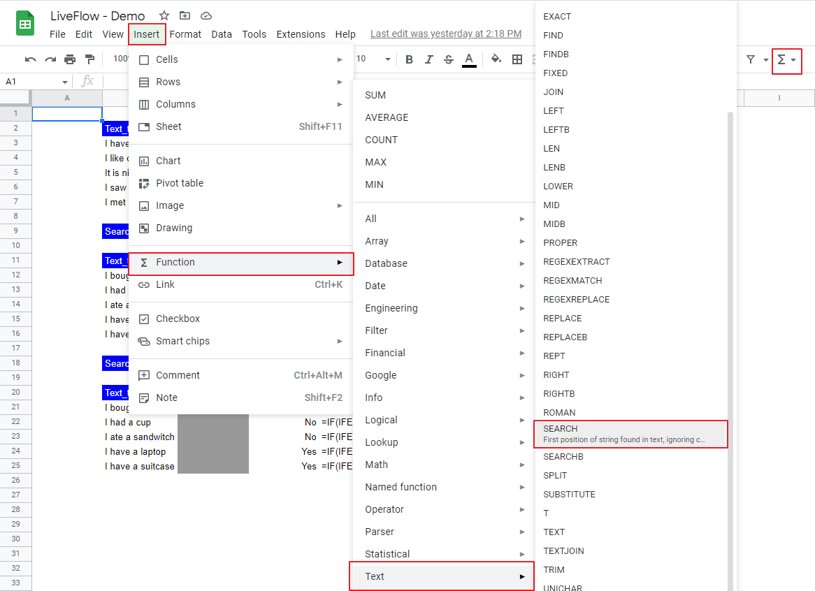
1. Type “=SEARCH” or go to “Insert” → “Function” (or directly navigate to the “Functions” icon)  → “Text” → “SEARCH”.
2. Specify a string you want to look up and text where the formula searches the specified string. If necessary, input at which the search starts (e.g., starting the search from the third letter in the selected text).
3. Press the “Enter” key.

‍

The general syntax of this formula is as follows:

SEARCH(search_for, text_to_search, [starting_at])

Search_for: a string you want to find in texts

Text_to_search: A text where this function looks for the specified keyword

Starting_at [Optional]: This argument determines where the search starts in the specified text. Without any input for this parameter, the function assumes it is 1 (=the first letter in the text string).

‍

Note: If the function can’t find a match, it returns “#VALUE”.

‍

Look at the following examples to understand how this formula works in Google Sheets.

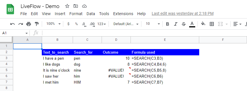
‍The first and second examples: The difference between the first and second examples is the optional argument “Sarting_at”. In the second formula, with 6 in the “starting_at” parameter, the search starts at the sixth position, “e” at the end of “I like”. Note that the SEARCH formula counts the location number at which the specified string shows up from the beginning of the text, regardless of the “starting_at” argument. 

‍

The third and fourth examples: The SEARCH functions return “#VALUE” in the third and fourth examples. In the third one, with 8 in the “starting_at” parameter, the function starts looking for “nine” from “e” (at the end of “nice”), a letter positioned at the tenth place in the text. However, after “e”, there is no chunk of letters that match with “nine”, so the function returns “#VALUE”. Similarly, the formula can’t find “him” in the specified text of “I saw her”, and it provides you with “VALUE” here. 

‍

This fifth example: The last example represents one of the features of this function. Although “him” and “HIM” are not the same, as the SEARCH formula is not case-sensitive, they are considered the same by the function. 

‍

You have learned how the SEARCH formula works in Google Sheets. We explain another example in which we use the SEARCH function combined with the IFERROR and IF formulas to check whether a specific string is included in a chosen text. In this sample case, assume that we confirm whether each text contains “have” or not.

The upper table describes the two steps you need to take. 

The first step is to use the SEARCH formula to confirm if “have” is contained in each text. In the “Outcome” column, we use the IFERROR formula to give a different value, “No”, to “#VALUE”, which shows up when there is no match in a search by the SEARCH function. 

The second step is to give the answers to the question.  In the “Include “have”?” column, we apply the IF function to show “No”, when the returned value by the IFERROR function is “No”, and otherwise, provide “Yes”, when the IFERROR formula gives us any numeric value.

‍

The lower table shows the same results in a step in which we use IF formulas containing two functions - the SEARCH and the IFERROR.

‍

These formulas are examples. Find a better combination of formulas that fit your purpose most.