
How to Use SUMIF Function in Google Sheets
In this article, you will learn how to use Google Sheets SUMIF Function.
What is the SUMIF formula in Google Sheets?
The SUMIF function in Google Sheets is useful when you want to sum a range of cells based on a specific criterion. It can save you a lot of time and make your spreadsheets more dynamic by automating the process of summing values based on specific criteria.
For instance, you can use the SUMIF formula when:
- Summing sales figures based on a specific value: If you have a sheet with a list of all your sales and the product sold in each sale, you could use the SUMIF function to quickly sum all sales for products whose sales are over a specific standard.
- Adding up the values in a range based on a specific date: If you have a sheet with a list of all your transactions and the date of each transaction, you could use the SUMIF function to quickly sum all transactions that occurred on a specific date.
- Summing the values in a range based on a specific category: If you have a sheet with a list of all your expenses and the category of each expense, you could use the SUMIF function to quickly sum all expenses that fall under a specific category.
Why is the SUMIF function in Google Sheets useful?
The SUMIF function in Google Sheets is a powerful and versatile tool that is useful for calculating the sum of values in a range of cells based on a certain requirement.
Here are some reasons why the SUMIF function is beneficial:
- Conditionally summing values: The SUMIF function allows you to sum values in a range of cells based on a specified condition. This can be helpful when you only want to sum values that meet a certain condition, such as summing all sales for a specific product, summing expenses for a particular category, or summing revenue for a certain date range.
- Flexibility: The SUMIF formula in Google Sheets is flexible and can be used with a wide range of criteria, including numbers, text, dates, logical expressions, and more. This makes it versatile for different types of data and criteria, allowing you to customize the summing operation based on your specific needs.
- Dynamic calculations: Like other formulas in Google Sheets, the SUMIF function is dynamic, meaning that if new data is added or existing data is modified and the SUMIF function is properly inserted, the sum will automatically update. This makes it convenient for handling changing data and ensures that the calculated results are always up-to-date.
- Efficiency: The SUMIF formula can be more efficient than manual calculations, especially when dealing with large datasets. It can quickly and accurately sum values that meet a particular criterion, saving time and effort compared to manually sorting and summing data.
- Error reduction: The SUMIF function can help reduce the risk of errors that may occur when manually summing values based on criteria. It eliminates the possibility of human mistakes, such as miscounting or omitting values, and ensures accurate and reliable results.
- Simplifying a formula: The SUMIF formula works as a combination of the SUM and IF functions. By reducing the number of formulas used in the calculations, you can make the calculation process simplified and clear.
In summary, the SUMIF function in Google Sheets is useful for conditionally summing values based on specific criteria, providing flexibility, dynamic calculations, error reduction and simplifying a formula.
How to add up numbers with a condition in Google Sheets
- You need to decide which cell you want to show the aggregated number.
- In the chosen cell, type “=SUMIF(” or select the function from a list of functions (Go to the “Insert” tab, move to the “Function”, click “Maths” and select the “SUMIF” function.)
- Enter three arguments; range, criterion, and sum range. You can directly type in these elements or use cell references.
- Press the “Enter” key on your keyboard.

The general syntax of the SUMIF formula is as follows:
range: This is the column the function refers to check if there is data that matches the criterion.
criterion: This could be a specific word/text, number, or date. You can input it directly in the formula or refer to a cell containing it.
sum range: This range should correspond to the “Range” regarding the number of cells and directions.
Note: The size of the range for the “range” argument must be the same as that of the “sum range” parameter.
How to use the SUMIF formula for a numeric criterion in Google Sheets
Look at the examples below. Assume you want to know the aggregated score for Division 1 based on the data set below. First, you need to select the “Division” column as “range”, reference cell C11 as “criterion”, and choose the “Score” column as “sum range”.
The formula in cell D11 returns 100 according to the arguments input. In cell D12, you can find another formula returning the same value, in which we use a manual input for the “criterion” argument. When you enter a numeric value in a parameter, you don’t need to enclose it with quotation marks.

Next, look at the examples in which you use a logical operator with a number in the “criterion” argument. This time, imagine you want to sum up scores for items with scores greater than 40. You can use the “<” operator.
We show the three types of formulas, which vary in terms of how to enter criterion, in the following screenshot: (i) cell reference referring to a cell, (ii) cell reference referring to two cells, one for a logic operator and the other for a numeric value, and (iii) a manual input. Note that you need to enclose a number with a logic operator with quotation marks, as shown below.

You can use the following signs to define the relationship between numbers in Google Sheets.
equal: =
larger than: >
smaller than: <
greater than or equal to: >=
less than or equal to: <=
not equal: <>
How do I sum cells with the specific text in Google Sheets?
You can sum cells based on the text as well. In the examples below, assume that you add scores for Division DEF. If you use the cell reference for the “criterion”, you can use the SUMIF formula as you use it for a numeric condition.
When you manually input a text criterion in the argument, the standard should be inside quotation marks, as shown in the picture below (cell D37).

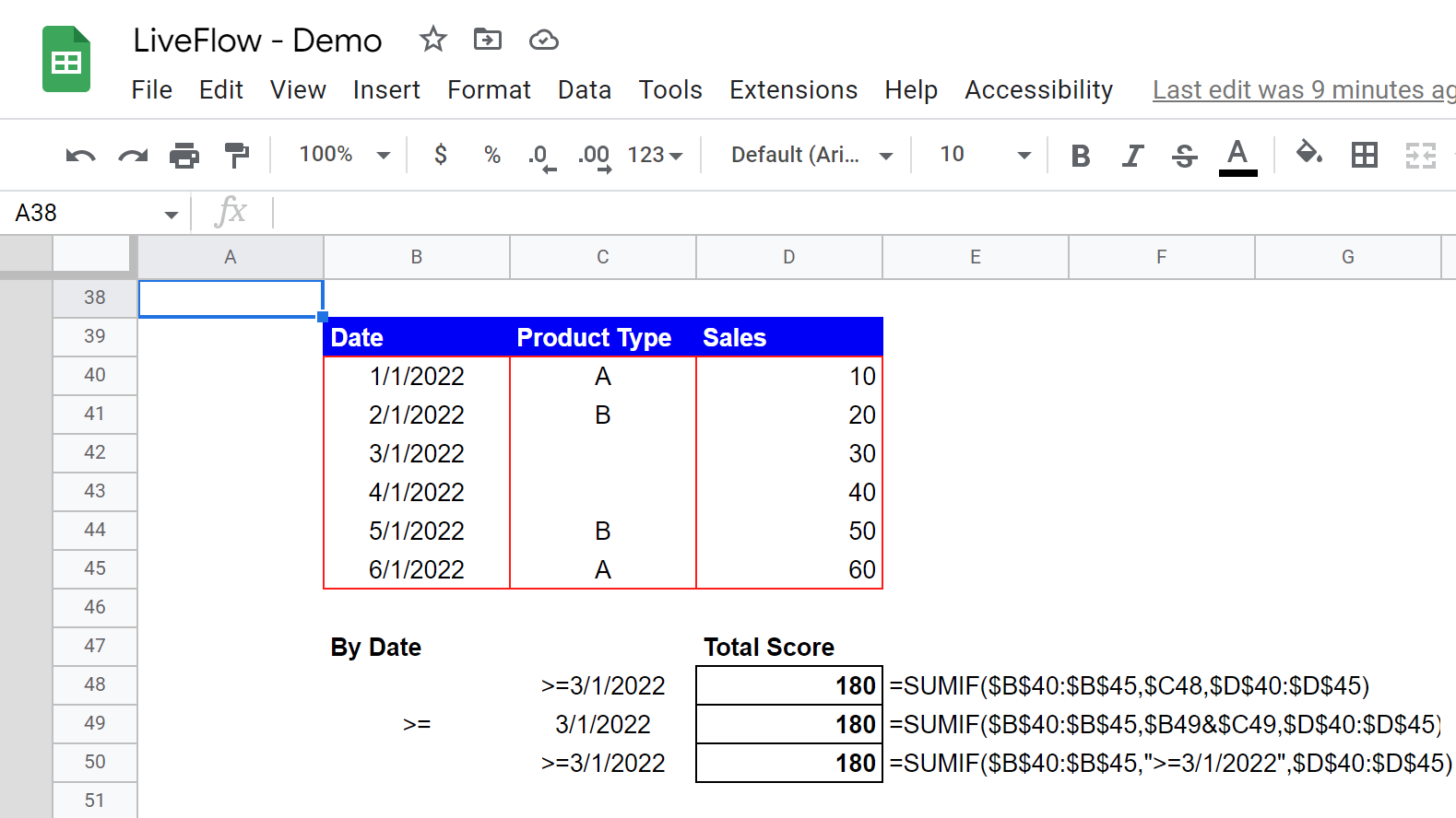
How to use the SUMIF formula for dates in Google Sheets
In this section, you will learn how to use the SUMIF function for dates. When you handle a date for this function, you can consider it similar to a text value.
Take a look at the following picture to see three patterns of inputs: (i) cell reference referring to a cell, (ii) cell reference referring to two cells, one for a logic operator and the other for a numeric value, and (iii) manual input.
Note that you need to enclose a number with a logic operator with quotation marks, as shown below.
How to use the SUMIF function for blank cells or non-blank cells in Google Sheets
Finally, learn how to aggregate numbers depending on whether a certain cell is blank. You can use one of the following logic operators: “<>” for non-blank cells or ““ for blank cells.
Imagine that you want to add up sales amount of items whose “Type” is unknown, or blank. In this case, you must enter ““ in the “criterion” argument. On the other hand, if you want to know the total sales amount for items whose “Type” are identified in the “Type” column, you can insert ““ in the formula, as shown in the following examples.

Can you use the SUMIF function with three criteria in Google Sheets?
Yes, you can, but you need to use the “SUMIFS” function for multiple criteria instead of the “SUMIF” function we introduce on this page. Check the following page to learn about the SUMIFS formula: SUMIFS Function in Google Sheets: Explained