SUMIF Function in Excel: Explained

In this article, you will learn how to use the SUMIF formula in Excel.

‍

How does the SUMIF formula work in Excel?

The SUMIF formula in Excel allows you to sum up a range of cells based on a specific condition. 

‍

When is the SUMIF function helpful in Excel?

The SUMIF function in Excel is helpful when you need to add up a range of cells based on a specific condition or criteria. This function can be beneficial in a variety of situations, such as

1. Totaling numbers based on a specific value: The SUMIF formula can aggregate numbers that meet a particular condition. For instance, you can total revenue from clients over $10,000 per month.
2. Aggregating values based on a date range: You can use the SUMIF formula to sum values based on a date range. For example, you could use SUMIF to compute total sales for a specific month.
3. Summing values based on a specific text: You can use the SUMIF function to sum values in a column based on a particular category in another. For example, you could use the SUMIF formula to add up all sales for a specific product category.

‍

How do you use the SUMIF formula in Excel?

The syntax for the formula is as follows:

=SUMIF(range, criteria, [sum_range])

"range" is the range of cells to which you want to apply the criteria to

"criteria" is the condition that must be met for the cells to be included in the sum. 

"sum_range" is the range of cells that you want to sum. This argument is optional, and if this is not specified, the "range" argument is used as “sum_range”.

‍

Note 1: When you input the “criteria” argument directly in the formula by typing it, note that any text criteria or any condition containing logical or mathematical signs need to be enclosed by quotation marks. If you enter a numeric standard, double quotation marks are not necessary.

Note 2: The ranges sizes for the “range” and “sum_range” arguments should be the same. Otherwise, the result provided by the formula may be incorrect, though it may still run the calculation. (The formula considers the “sum_range” as a range starting from the first cell in the “sum_range” but having the same dimension as the range specified in the “range” argument.

‍

How to use the SUMIF function with a numeric condition

Before looking at sample SUMIF formulas containing numeric criteria, get yourself familiarized with logic operators, such as “>” (greater than) and “<” (less than).

1. >N: Greater than N
2. >=N: Greater than or equal to N
3. <N: Less than N
4. <=N: Less than or equal to N
5. =N: Equal to N
6. <>N: Not equal to N

Assume you have the dataset in the picture below and want to compute the Total Sales amount that meets a specific criterion, such as Total Sales from clients with Sales over 5,000. The formula and its arguments are as follows:

=SUMIF($E$3:$E$12,”>5000”,[$E$3:$E$12])

"range": $E$3:$E$12

"criteria": ”>5000”

"sum_range": $E$3:$E$12 (This can be omitted in this case)

You can see other examples in the screenshot below as well. Note that when you use an equal operator “=” with a specific number, you can directly input the particular number without the operator, as shown in the fifth example formula below.

‍

How to use the SUMIF function with a date condition

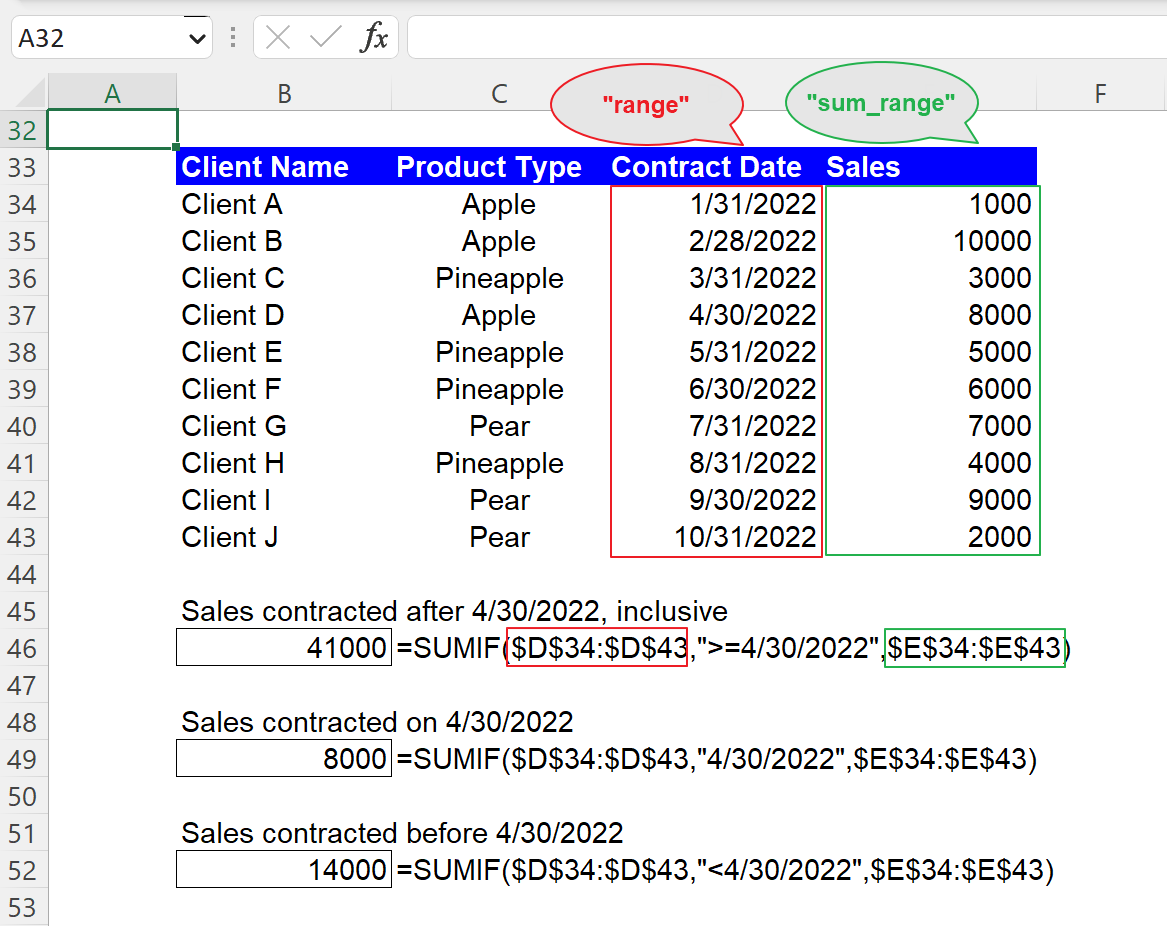
You can use a date as the “criteria” argument in the SUMIF function, almost similar to a number criterion. So, you can combine logic operator(s) with a date to create a condition. However, note that you need to enclose a date with quotation marks when you directly enter it in the formula, such as the following formula:

=SUMIF($D$34:$D$43,”>=4/30/2022”,$E$34:$E$43)

"range": $D$34:$D$43

"criteria": ”>=4/30/2022”

"sum_range": $E$34:$E$43 (This can’t be omitted in this case)

You can see two more sample formulas with date conditions in the following picture.

‍

How to use the SUMIF function with a text condition

You must remember that when you manually insert a text condition as the “criteria” argument, you always need to enclose them with double quotes. Also, you can use the operators, such as “<>” or the wildcards, such as “*” and “?” together with a text string to form a condition. For example, if you want to calculate the total sales amount from the product “Apple”, you can apply the following formula to the dataset.

=SUMIF($C$56:$C$65,”Apple”,$E$56:$E$65)

"range": $C$56:$C$65

"criteria": ”Apple”

"sum_range": $E$56:$E$65 (This can’t be omitted in this case)

You should bear in mind that this formula is not case-sensitive. So, for example, you can get the same result when you use “apple” instead of “Apple” as “criteria” in the formula. The picture contains four more sample SUMIF formulas with text conditions if you are interested.

‍

How to use the SUMIF formula with cell reference

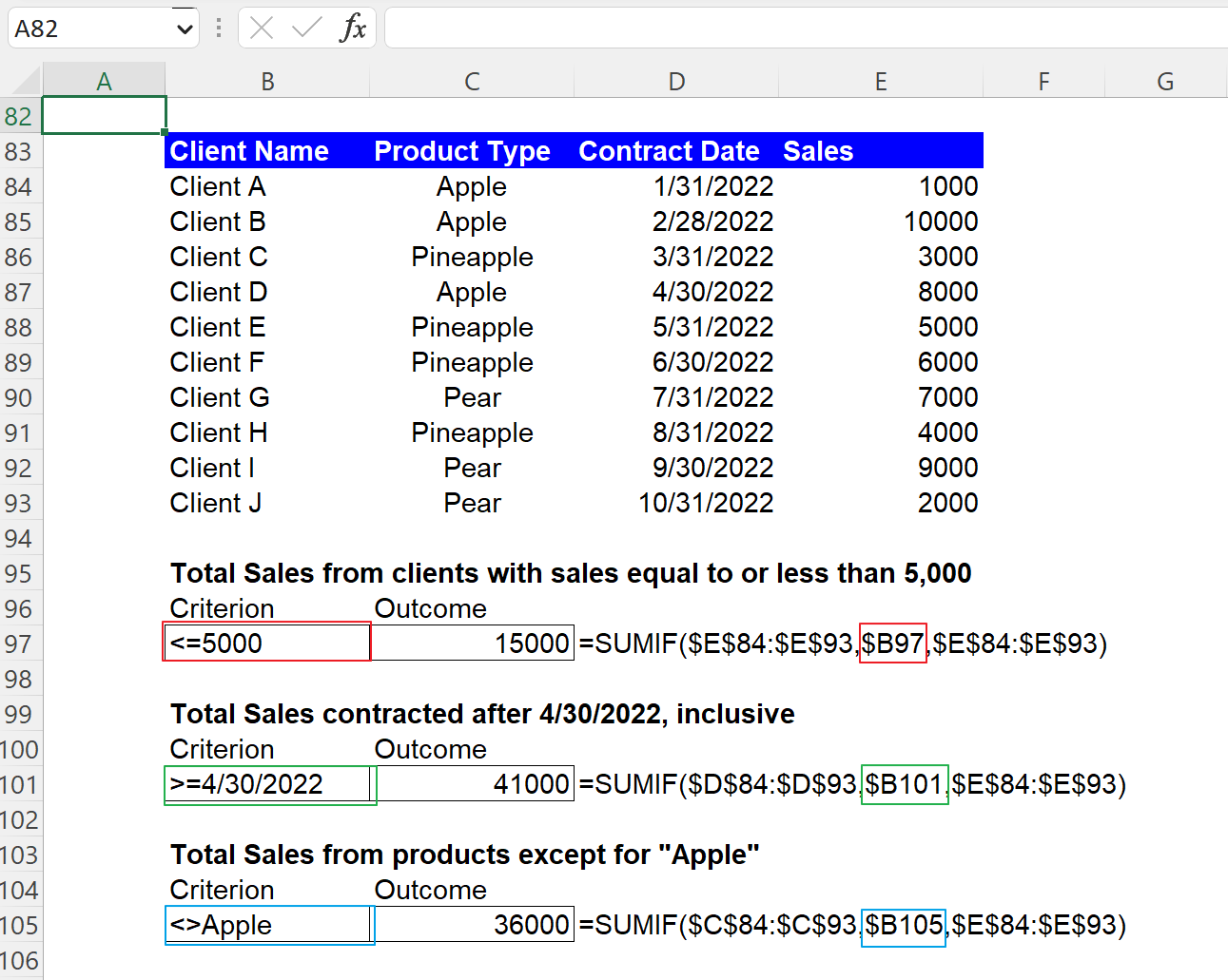
Although you can manually enter “criteria”, as shown in the examples above, instead, you can use the cell reference to input the “criteria” argument. We recommend the cell reference approach because it gives you more visibility and clarity about the condition as the requirement can be seen in a cell and allows you to change the condition more quickly. You don’t need to put your cursor on the cell containing the formula or open the cell by hitting the F2 button to see in detail or revise the function. Note that you don’t need to enclose it with quotation marks when you put a criterion in a cell, as shown in the picture below.

‍

What is the difference between the SUMIF and SUMIFS functions in Excel?

Both the SUMIF and SUMIFS functions in Excel are used to sum a range of cells based on one or more conditions, but the main difference between the two functions is that the SUMIFS formula allows you to use multiple criteria to sum a range of cells, while the SUMIF function enables you to use only one criterion. In this regard, we could say the SUMIFS function is more versatile and flexible, allowing you to use multiple conditions to aggregate a range of cells, while the SUMIF formula is more straightforward and explicit but less flexible, only allowing you to use one requirement.

‍

Analyze your live financial data in a snap in Google Sheets

Are you learning this formula to visualize financial data, build a financial model, or conduct financial analysis? In that case, LiveFlow may help you automate manual workflows, update numbers in real-time, and save time. You can access various financial templates on our website, from the simple Income Statement to Multi-Currency Consolidated Financial Statement. Are you interested in this product but are an Excel user? That’s not a problem at all. You can connect Google Sheets to Excel quickly. 

To learn more about LiveFlow, book a demo.