
Pivot Table in Google Sheets: Explained
In this article, you will learn what a pivot table is and how to use it in Google Sheets.
What is a pivot table used for?
A pivot table allows you to organize, summarize and analyze data.
If the amount of data you are looking at is small, a function and/or a filter or filter view may be enough to arrange and analyze the data. However, suppose the volume of information is significant. In that case, a pivot table is recommended because it is easy and quick to use.
Still, it equips many functions, such as calculating average sales amount by person, showing the number of deals by region, and so on. You can create a pivot table by following suggestions from Google Sheets or manually.
How to create a pivot table in Google Sheets
Creating a pivot table based on Google Sheets’ suggestions
- Select a data set you want to examine.
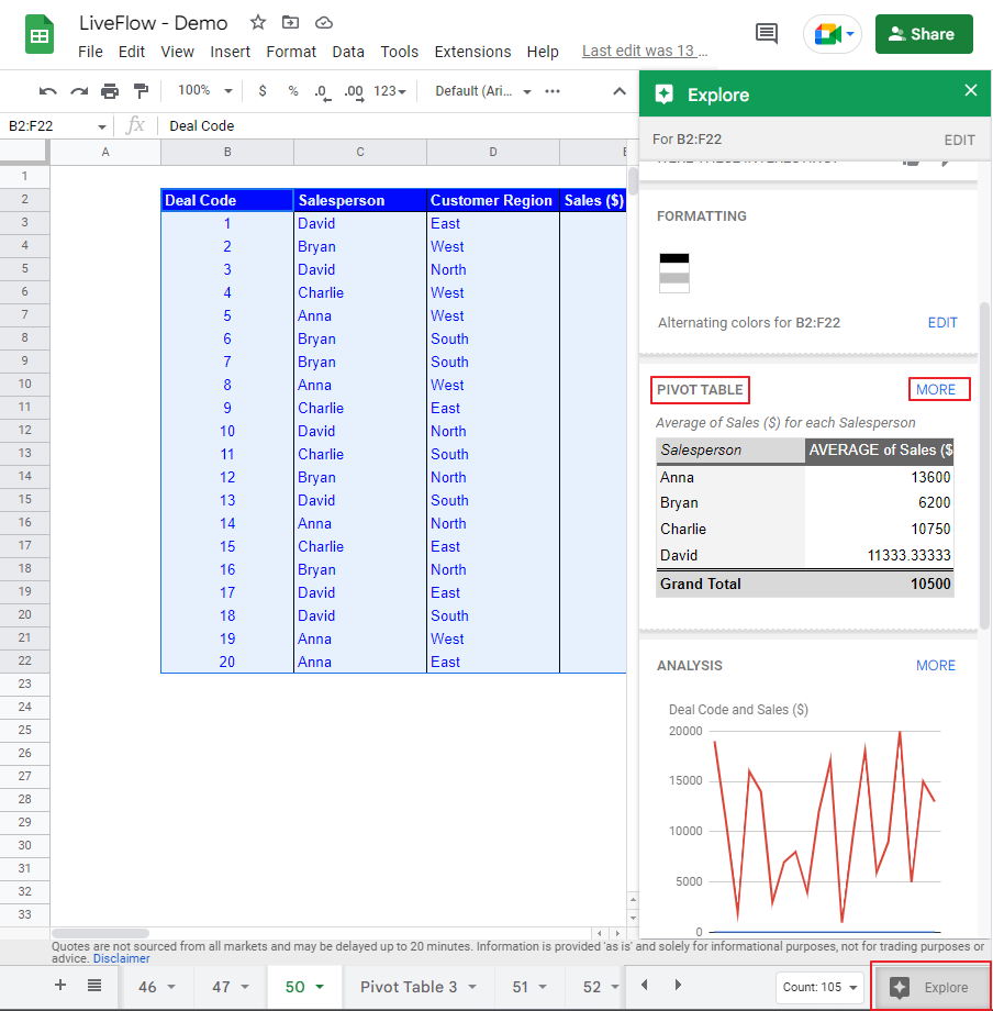
- Navigate to the “Explore” icon at the bottom right of a sheet.
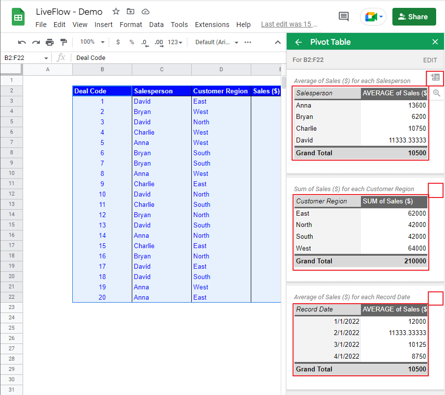
- Go to the “PIVOT TABLE” section → click “MORE” at the top right of the section to see all suggestions.
- (4-a) Click the “Insert Pivot Table” icon at the top right of each output image, or (4-b) click an output image → Click the “Insert Pivot Table” icon at the top of the pop-up window.
- Determine if you insert the table on a new sheet or one of the existing sheets. If you add a pivot table on an existing sheet, you need to specify a range.
- Click the “Create” button.
Step 1 to 3
Step 4
Step 5 and 6
Creating a pivot table manually
If you don’t find an ideal pivot table in Google Sheets’ suggestions, you can make a pivot table by yourself.
- Select a data set you want to examine.
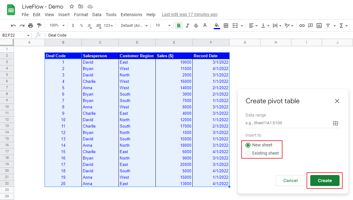
- Move to the “Insert” tab → “Pivot table”.
- Determine if you insert the table on a new sheet or one of the existing sheets. If you add a pivot table on an existing sheet, you need to specify a range.
- Click the “Create” button.
Step 1 and 2

Step 3 and 4
How to use a pivot table function in Google Sheets
Learn how to create a pivot table with an example.
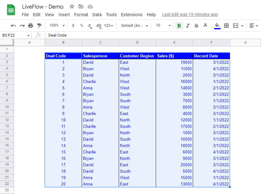
Assume you have the following data. You want to know the sum of sales for each salesperson quickly. First, make a pivot table manually by following the steps described above.
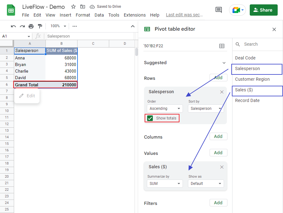
When you insert a pivot table, you will see the frame at the top left corner of the sheet and the “Pivot table editor” on the right side.
In the editor, you can see (i) the selected data range, ‘50’!B2:F22 in this example, (ii) Suggested pivot tables, (iii) “Row”, “Column”, “Values”, and “Filters”, which correspond to those in the frame, except for “Filters”, and (iv) table headers in the source data table, such as “Deal Code”, and “Sales Person” on the right side of the editor.
To generate a table, you must assign the items to the appropriate locations. When you set an item in the “Row”, “Column”, “Values”, or “Filters”, you can click the “Add” button next to each section name or drag an item from the list and drop it onto one of the sections.

Recall we are trying to make a summary table showing the sum of sales for each person.
- Allocate “Sales Person” in the “Row” section.
- Put “Sales ($)” in the “Values” section.
As you can guess from the picture below, you can adjust the create table by changing choices in drop-down lists in the selected items. In this case, for “Salesperson” in the “Row” section, you can change the order of names (e.g., ascending or descending) and the way of sorting (e.g., Salesperson or Sum of Sales ($) amount). By checking the box next to “Show totals”, you can add a row at the bottom of the table.
For “Sales ($)” in the “Values” section, you can select how you show the values. By switching the “Summarized by” pull-down menu, you can use other functions such as COUNT and AVERAGE instead of SUM. You select a different format in the “Show as” pull-down menu, such as “% of row”, “% of column”, or “% of grand total”.
Next, imagine you need to see the sum of Sales ($) by salesperson and customer region. Also, as David is no longer in your company, you want to see only the other three salespersons.
- Add “Customer Region” to the “Column” section.
- Set “Salesperson” in the “Filters” section.
- Click the drop-down list in the “Filters” section and uncheck “David”.
You can make changes to the added items, “Customer Region” in the “Column” section and “Salesperson” in the “Filters” section. In the “Column” section, you can make similar adjustments to what you can do in the “Row” section.
In the “Filters” area, you can use it the same way as a filter in a worksheet. Note that you can delete the item from each section by clicking the “X” sign at the top right corner of each item and that you can assign more than one item to each section if necessary.

You can create a table shown by using basic functions SUM and SUMIFS but utilizing a pivot table is quicker and easier.
Consider making a pivot table next time you need to summarize, organize or analyze a certain amount of information and save time.
Do pivot tables automatically update Google Sheets?
Yes, they do, as they are dynamic. Once you change the original data, the changes are immediately reflected in a pivot table. However, you should be careful in the following cases.
- You put a filter in a pivot table. You need to remove the filter and then add the filter again to reflect the additional data.
- You add a new row or column out of the selected range for a pivot table. You must include the additional row or column in the chosen field in the “Pivot table editor”.
- If the original data includes functions such as NOW and TODAY, then they will not be shown in a pivot table in real time. The way to avoid it is to not include those formulas in an original data set.
Wondering how to automate your custom Pivot tables and bring live QuickBooks Online data in? Check LiveFlow. It will connect live data and update any table as you need it. Here’s an example:


