How to Use PRODUCT Function in Excel (User-friendly Tutorial)

In this article, you will learn how to multiply numbers and calculate products in Excel using the PRODUCT formula.

‍

Understanding the PRODUCT formula in Excel

The PRODUCT function in Excel is used to calculate the product of the selected values. In other words, it multiplies each of the values selected in Excel.

‍

The PRODUCT function syntax in Excel

=PRODUCT(number1, [number2], ...)

In the above syntax, each number selected will be multiplied and the result will be displayed.

For example: if 5 is number 1, 6 is number 2 and 10 is number 3, the formula =PRODUCT(5,6,10) will calculate the product value to be 300.

‍

Usage of the PRODUCT formula in Excel

The PRODUCT function in Excel can be used for the following use cases:

Derive total revenue: If you have a list of products with their prices and quantities, you can use the PRODUCT formula to calculate the total revenue by multiplying the prices with the quantities sold.

Forecast based on growth rates: If you have data on the revenue of a business and wish to project its growth trajectory over a period, you can use the PRODUCT function in Excel to multiply the revenue into the growth rate for multiple forecasted periods.

Calculate compound interest: If you want to calculate the compound interest on an investment, you can use the PRODUCT formula to multiply the principal amount, interest rate, and the number of compounding periods.

Ascertain the total cost of a project: If you have a list of tasks with their durations and costs, you can use the PRODUCT function in Excel to calculate the total cost of the project by multiplying the duration with the hourly rate or cost per task.

‍

Inserting the PRODUCT function in Excel

Step 1: Type “=PRODUCT” in the cell where you want to derive the result

Step 2: Once the formula prompt opens up, click on the PRODUCT formula

Step 3: Select the values one by one by separating them with “,” (commas) as shown in the image below

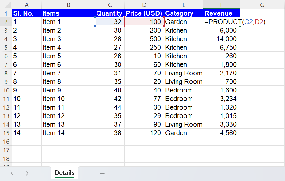
‍Step 4: Press the “ENTER” key

‍

Note 1: The PRODUCT function in Excel can be replaced with the “*” (asterisk) sign, which denotes the mathematical operation of multiplication. For example: “=C2*D2” will give you the same result as “=PRODUCT(C2,D2)”.

Note 2: The PRODUCT function can also be used as an array formula. For example: “=PRODUCT(A1:A5)” will multiply each of the values in cell A1,A2, A3, A4 and A5.

Note 3: Only numeric values are multiplied with the PRODUCT formula. Blank cells, logical values, text strings or any references are ignored.

‍

Analyze your live financial data in a snap in Google Sheets

Are you learning this formula to visualize financial data, build a financial model, or conduct financial analysis? In that case, LiveFlow may help you automate manual workflows, update numbers in real-time, and save time. You can access various financial templates on our website, from the simple Income Statement to Multi-Currency Consolidated Financial Statement. Are you interested in this product but are an Excel user? That’s not a problem at all. You can connect Google Sheets to Excel quickly. 

To learn more about LiveFlow, book a demo.

You can learn about other Excel and Google Sheets formulas and tips that are not mentioned here on this page: LiveFlow‘s How to Guides