How to Use Data Validation in Google Sheets
[This article was updated on March 2nd, 2023]
In this article, you can get yourself familiarized with the Data Validation function in Google Sheets.
What is the Data Validation in Google Sheets?
Data Validation in Google Sheets is a feature that allows you to control the type of data that users can enter into a cell or range of cells in a sheet. When a user tries to enter data that doesn't meet the validation criteria, Google Sheets will display an error message and prevent the user from entering the incorrect data.
This can help avoid errors and ensure the accuracy of your worksheet data and formulas. For example, with data validation, you can set rules to restrict the type of data that can be entered into a cell, such as:
- A specific number range, such as only allowing numbers between 1 and 100
- A list of predefined values or text strings, such as only allowing the values "Yes" or "No"
- A specific date range, such as only allowing dates within a certain period
When would you use the Data Validation in Google Sheets?
By leveraging the Data Validation function, you can make your analysis, a KPI dashboard, or a financial model more efficient and valid without overlooking irregular input or revising your model or formulas to adjust to new input types.
More specifically, for instance, Data Validation is beneficial in the following occasions:
- You want to keep data input consistent in a list from the beginning to the end.
- You would like to limit data input (e.g., specific range of numbers: 1-10) or data style.
- You need to create a drop-down list that contains specific choices.
What was updated for the Data Validation function in Google Sheets?
In December 2022, two significant updates in Data Validation in Google Sheets occurred.
- Dropdown chips: Drop-down chips are a pull-down list feature that allows you to show and see the project statuses at a glance. Google Sheets had been equipped with the feature to create a similar drop-down list before the update, but this feature was enhanced to make it consistent with what had been available in Google Docs.
- Improved visibility of all data validation rules: Before the update, it was not necessarily easy to see all data validation rules at a glance. However, with the update, you can see all data validation rules in a list as you can do for the other features, such as Conditional Formatting, Protected Range, and Named Ranges. This improvement helps you manage the data validation rules more efficiently and accurately.
How to use Data Validation in Google Sheets
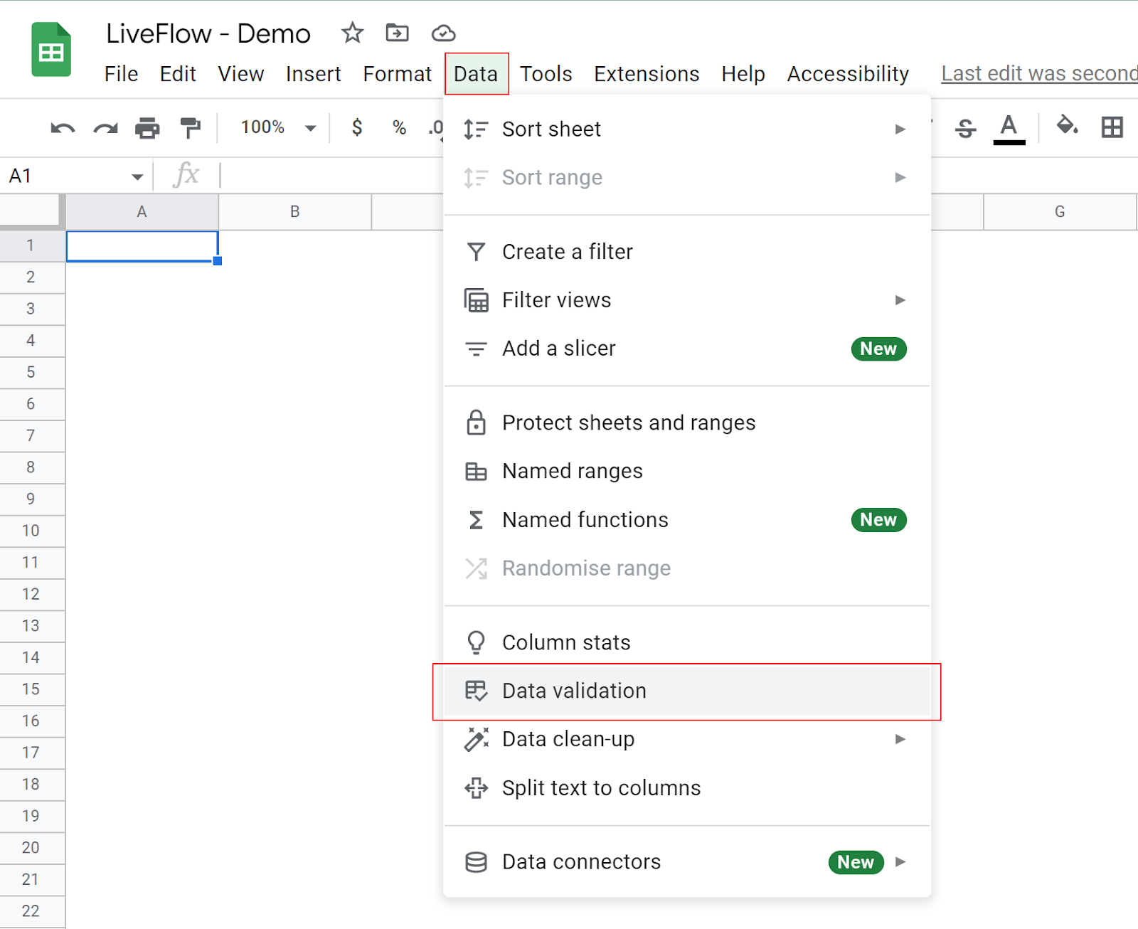
- Go to the “Data” tab, click “Data Validation”, and get a dialog box on the right side of the sheet.
- Click “+ Add rule”.
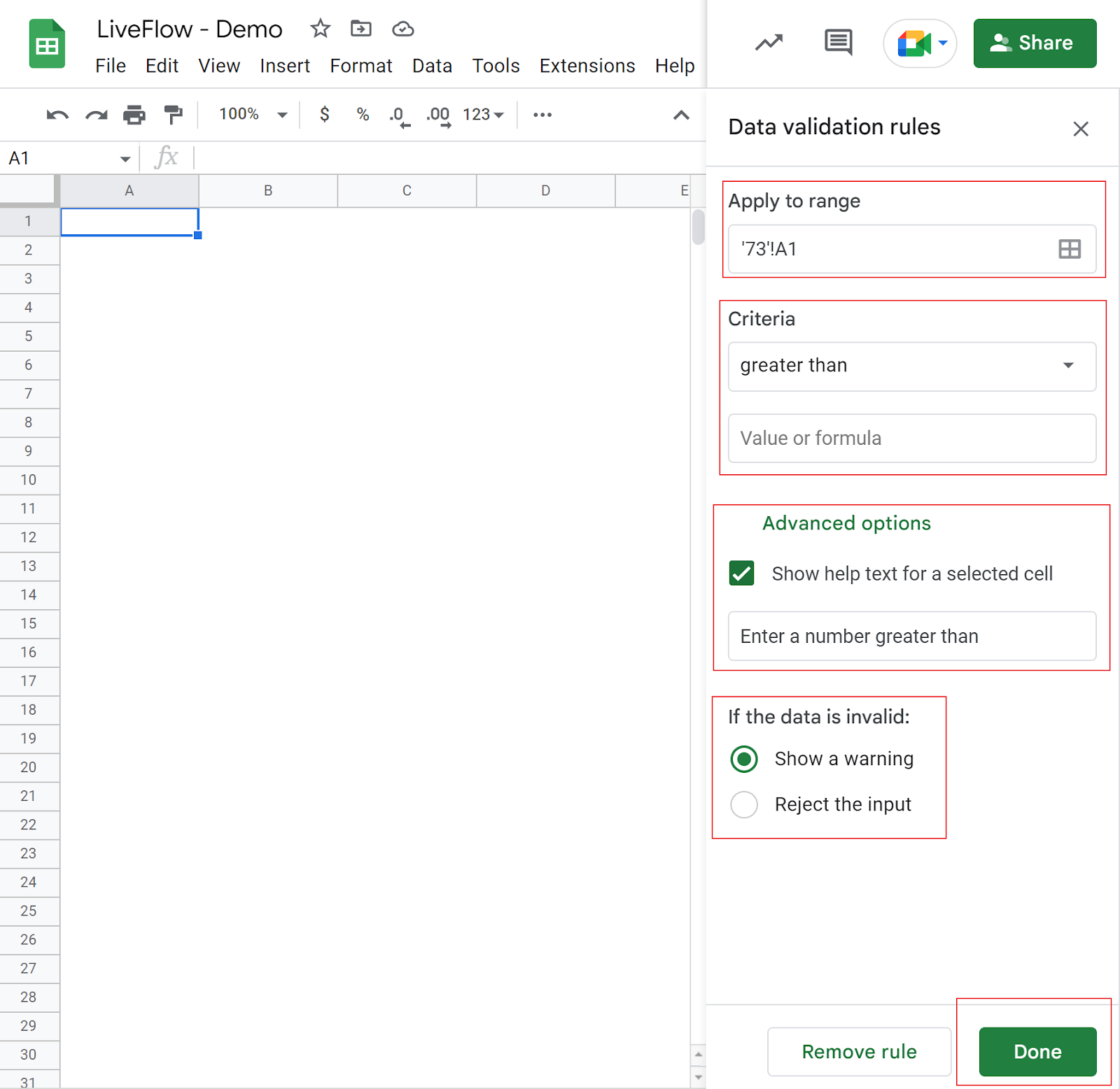
- Select a range where you want to make Data Validation effective.
- Choose one of the criteria and input values according to the criterion.
- Check the advanced option of “Show help text for a selected cell”, if you want to leave a hint to an editor who makes an invalid data input to make it valid.
- Choose one of two options* against invalid data input.
- Click “Done” to make the setting effective.
* ”Show a warning”: This option allows editors to input invalid data in a cell in the selected range but gives them a warning message that their inputs breached the defined input rule.
* “Reject the input”: This option refuses any invalid input.
Next, we will explain the types of data validation available in Google Sheets.
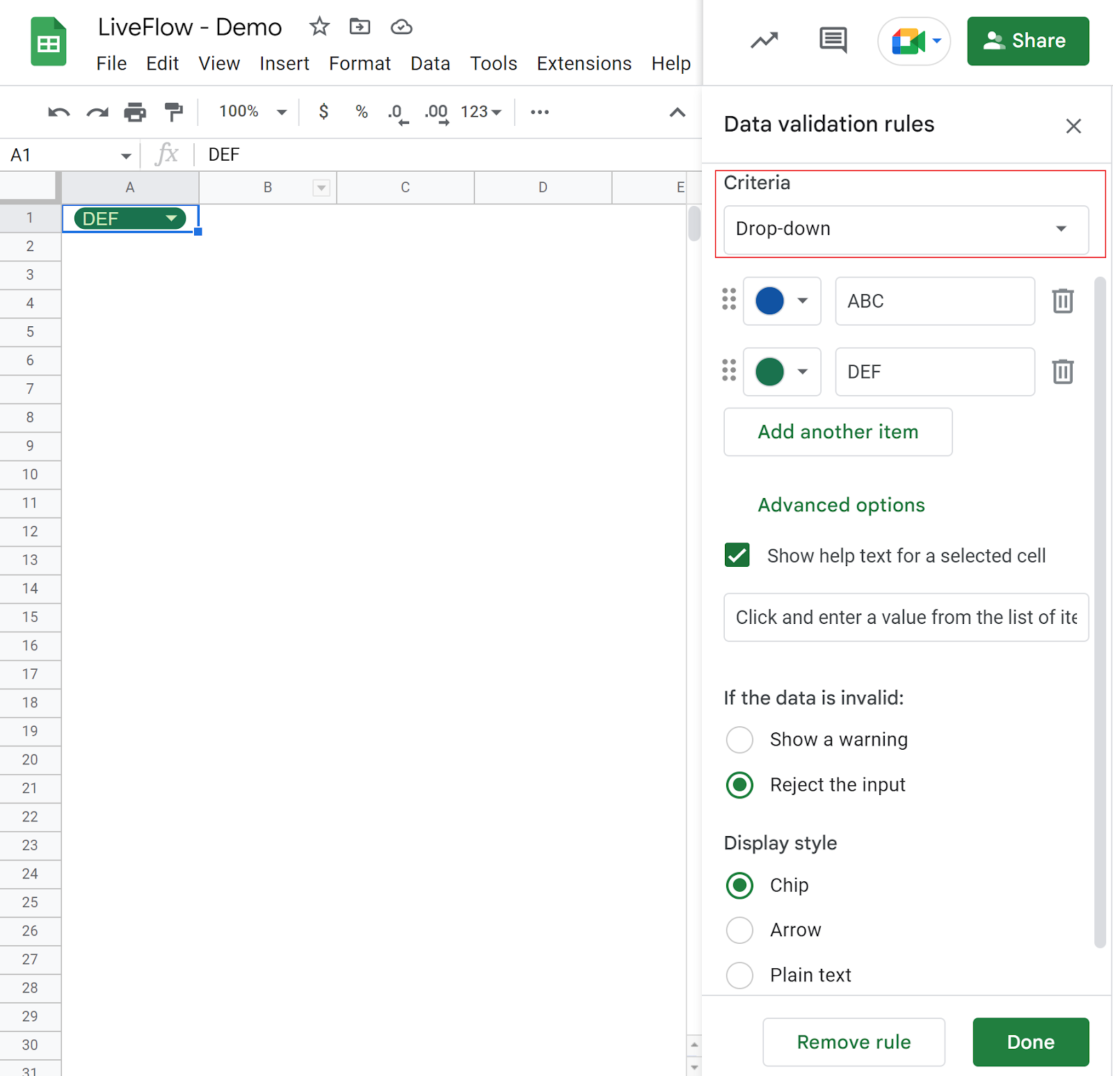
(i) Drop-down: This is the option to create a pull-down menu in the sheet by inputting the choices manually. You can assign a color to each alternative you generate.
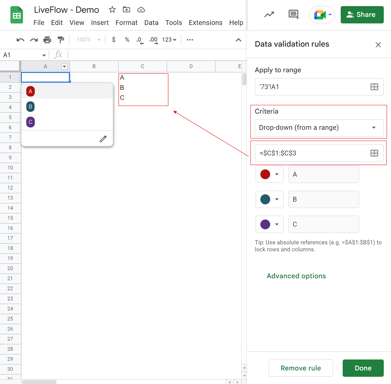
(ii) Drop-down (from a range): The only difference between drop-down and drop-down (from a range) is that the choices in the latter list are generated by cell references instead of manual input in the former list.
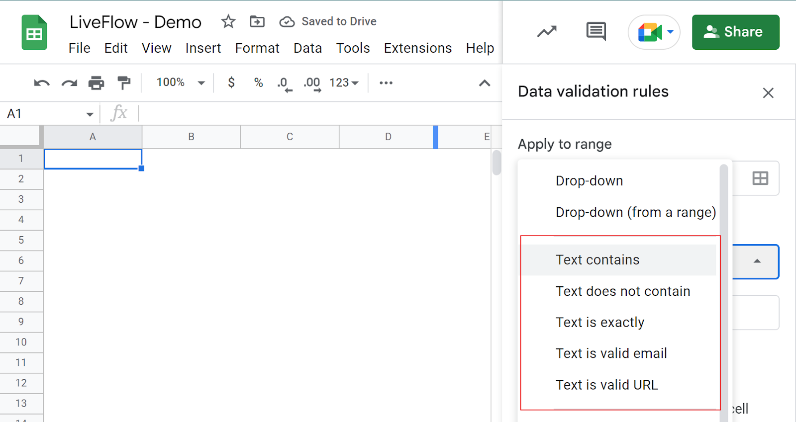
(iii) Text-related data validation: By selecting this option, you can limit the data input to text with conditions. There are five pre-fix conditions, “Text contains”, “Text does not contain”, “Text is exactly”, “Text is valid email”, and “Text is valid URL”. Note that, depending on the choice, you must input a specific text string in the text box.
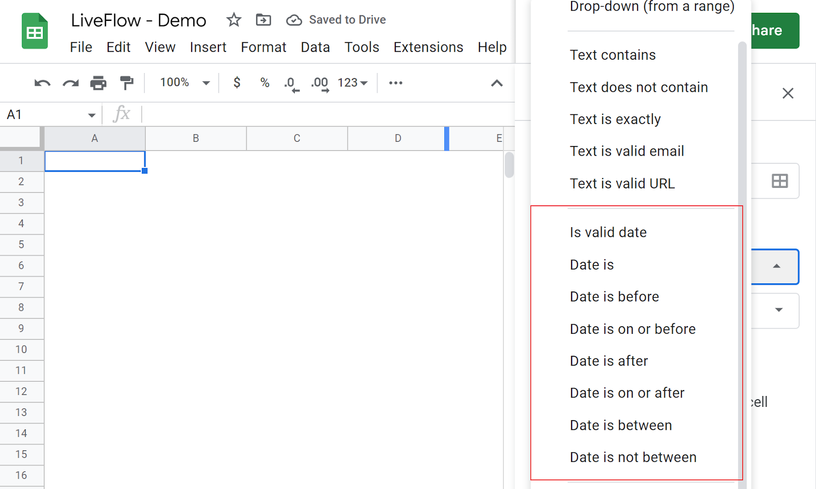
(iv) Date: If this is effective in a cell, the data input for the cell should be a date. There are eight pre-fix conditions about the date available. Similar to (iii) text, depending on your choice, you need to provide a specific date in the text box.
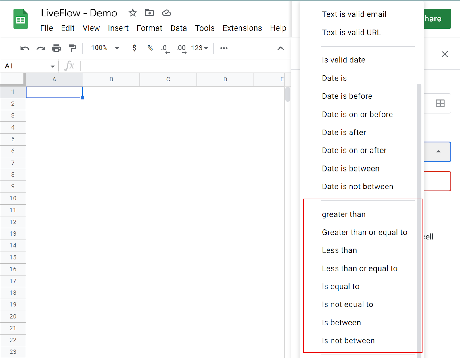
(v) Number: If you choose this, the input should be a certain numeric value or a formula. You can set up a condition such as “between X and Y”, and “greater than Z” out of the eight choices available.
(vi) Custom formula is: This option allows you to insert a formula to pull data from somewhere else.
(vii) Tick box: You can check or uncheck a box in a cell if you choose this option. You can enter a cell value corresponding to a checked box and another for an unchecked box. (e.g., TRUE for a checked box and FALSE for an unchecked box).
How do you insert a drop-down list and a tick box quickly in Google Sheets?
In addition to the way we introduced above, there is a quicker way to insert a drop-down list or a checkbox in Google Sheets.
- Navigate to the menu bar.
- Click “Insert”.
- Select “Tick box” or “Drop-down”.
- Then, the data validation rule pops up on the right side to edit the details.

How do I create a dependent drop-down list in Google Sheets?
To learn how to make a drop-down list in detail, refer to this article: Drop Down List in Google Sheets: Explained.
Also, if you are interested in creating a dependent pull-down list, in which the choices change according to a choice made in another drop-down list, you can learn it here: Dependent Drop-down List in Google Sheets: Explained.
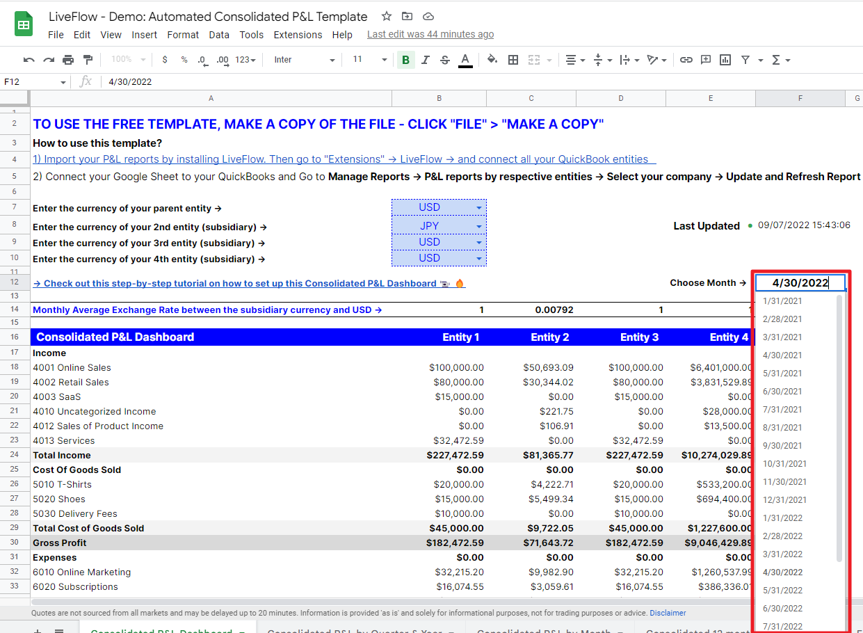
Finally, here is an example of a drop-down. This is LiveFlow’s Consolidated P&L Template For Excel & Google Sheets. You can see a drop-down list, with which you can switch monthly financial data, in the middle of the picture (the cell next to the text “Choose Month”).