How to Add Borders in Google Sheets
Would you like to make your table more visible and beautiful? It’s not difficult to do at all. In this article, you can learn how to add borders in Google Sheets.
What are borders in Google Sheets?
In Google Sheets, borders are lines that can be added to cells or ranges of cells to create a visual separation between them. Borders are a formatting option that can be applied to cells, columns, rows, or a range of cells. There are different types of borders available and change their color and thickness depending on your purpose.
Why do you add borders in Google Sheets?
There are several reasons why you may want to add borders in Google Sheets:
- Improve readability: Borders can help to separate different sections of data and make it easier to read and interpret. Also, adding borders can make your sheet look more professional and sophisticated.
- Highlight important information: You can use borders to draw attention to specific cells or ranges of cells that contain important information.
- Make data entry easier: Borders can be used to highlight cells where you need to input, combined by other Excel features, such as font color change and cell fill color change.
How do you make a border in Google Sheets?
Here is the answer to how to add cell borders in Google Sheets. Please refer to the screenshot below while reading.
- Open your Google Sheets.
- (After you input your content), select a range you would like to draw a border.
- Click the “Borders” icon in the toolbar.
- If you want to change border color and/or style, please click the border color icon and/or the border style icon in the detailed menu.
- Choose a pattern of a border you would like to apply to the selected range.
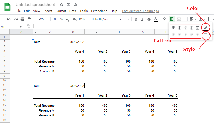
For your better understanding, let’s see the example of a design change, turning the upper table to the lower table, a more beautiful table with borders in the above picture.
- Select cell D2 and choose “Outer Border”.
- Select B6 to H6, and choose “Top Border” and “Bottom border”.
- Finally, select cell B4 to H4, change the border style to a bold one first, and then choose “Bottom border”.
Don’t you think that the table looks more beautiful and easier to follow?
Don’t like the border you applied? Just clean them up with the “Undo” function in the top left corner.
When you can’t use the “Undo” function (for example, when you make a lot of changes after you added borders), you can choose the “Clear border” pattern and apply it to a selected range.
How do I make white borders in Google Sheets?
- Select cells you want to add white borders.
- Go to the toolbar, click the “Borders” icon.
- Click the “Border color” icon (top right icon among the options), choose white from the list of colors.
- Select one of the border patterns from the list and click it.
How do you make thick borders in Google Sheets?
- Select cells you want to add thick borders.
- Go to the toolbar, click the “Borders” icon.
- Go to the toolbar, click the “Border style” icon (bottom right icon among the options), choose the third line from the top.
- Select one of the border patterns from the list and click it.

