How to Use SUM Function in Google Sheets
In this article, we will explain how to add numbers in some cells or in a selected range or array with a formula called “SUM.”
What is the SUM function in Google Sheets?
The SUM function in Google Sheets calculates the sum of a range of cells. It takes a cell, range, or array as arguments and returns the sum of the values in the specified area. The SUM function is beneficial whenever you need to calculate the total of a range of cells quickly. It is handy when you have a large data set and want a quick data summary.
For example, if you have a spreadsheet containing a list of expenses and want to know the total amount spent, you can use the SUM function to add up all the values in the "Amount" column.
Why is the SUM formula beneficial in Google Sheets?
Using the SUM function in Google Sheets can be beneficial for several reasons:
- Accuracy: The SUM function in Google Sheets ensures accurate calculations. It performs the addition operation automatically and eliminates the possibility of human errors that may occur when adding up numbers manually. This helps prevent mistakes in calculations and ensures accurate results.
- Efficiency: The SUM formula is designed to handle calculations on a large scale and across multiple cells or ranges. This makes it efficient for adding up numbers in columns, rows, or other ranges of cells, especially when dealing with large datasets. It can save time and effort compared to manual calculations, especially when dealing with complex or extensive data.
- Dynamic calculations: The SUM function in Google Sheets is dynamic. If new numbers are added to the range or existing numbers are modified, the sum will automatically update if it is properly inserted. This makes it convenient for handling changing data or scenarios where calculations need to be adjusted on the fly. It saves the hassle of manually updating calculations every time data changes.
- Collaboration: The SUM function is compatible with Google Sheets' collaborative features, allowing multiple users to work on the same sheet simultaneously. This makes it convenient for teams or groups to collaborate on calculations, share data, and review or verify calculations in real-time.
In summary, using the SUM function in Google Sheets can provide benefits such as accuracy, efficiency, dynamic calculations, and collaboration, making it a valuable tool for various tasks that involve adding up numbers and calculating totals in a spreadsheet environment.
How to use the SUM formula in Google Sheets
- Select a cell to show an aggregated number of values.
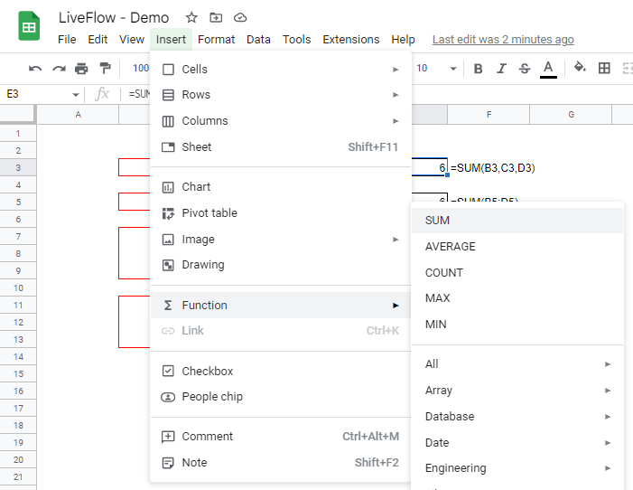
- In the chosen cell, type “=SUM(” and select cells or a range you want to sum up, or by choosing from a list of functions (Go to the “Insert” tab, move to the “Function”, and select “SUM” function.
- Then, you can manually type in values or input cells or a range by cell reference.
- Press the “Enter” key on your keyboard.
The general syntax of the SUM formula is as follows:
value1: This is the first number(s) to be added up
value2 (Optional): You can insert arguments up to thirty
How to add up cells in Google Sheets
If you want to sum up a couple of numbers without any functions, you can calculate the results, using the plus signs in the screenshot above. To add numbers in cells B2, C2, and D2, and show the result in cell E2, you can type “=B2+C2+D2” by manually inputting or selecting cell B2 and pressing the “+” mark and do the same for other cells (C2 and D2).
You can receive the same return by using the SUM function. To do so, insert the SUM formula and select three cells you want to add, separating them with commas, as shown in the picture below.

How to add rows in Google Sheets
As described above, you can select a row or rows as argument(s) in the SUM formula.
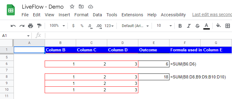
If you want to sum up numbers in Row 6 (from Columns B to D), you can define the formula as follows:
If you want to sum multiple rows, for instance, Row 8, Row 9, and Row 10 (again, from Columns B to D), you can create the formula below.
How do I make columns added up in Google Sheets?
As described above, you can select a column or multiple columns as parameter(s) in the SUM function. Enter the arguments similar to when you add up rows, which is described above.
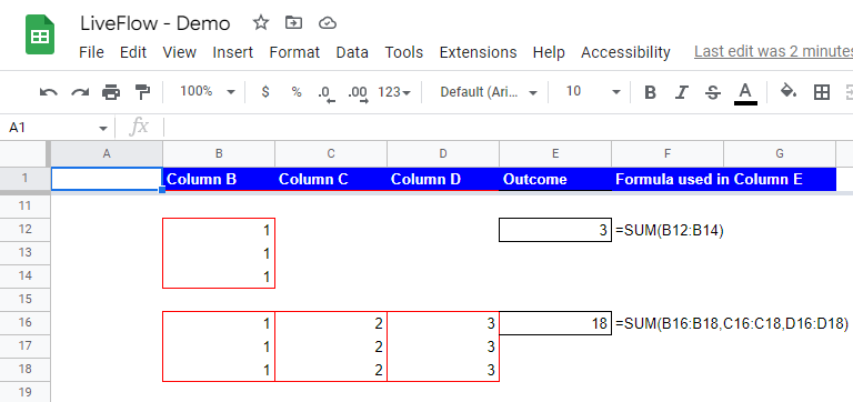
When you add up values in a column, you can select a range in a column as the following formula.
As another example, assume you want to sum up numbers in multiple columns, Column B (from Row 16 to 18), Column C (from Row 16 to 18), and Column E (from Row 16 to 18). You can define the formula as follows:
How to sum up values in an array in Google Sheets
Imagine you need to aggregate figures in a 3x3-sized array. When you sum up numbers in an array (or arrays), you can use the SUM function. For example, if you want to calculate the total number of values in the array of B20:D22, the SUM function would look like the one below.

How do you add up numbers automatically in Google Sheets?
If you in advance select a range including cells that you will fill in with numbers later, when you input any numbers in any cells in the selected range, all numbers are summed up automatically by the SUM formula. For example, let’s assume that you set the SUM formula “=SUM(B20:D22)”, and all cells in the range are blank.
If you input any figures in the range later, the numbers typed in are automatically summed up, and you can see the aggregated number in the cell you input the formula (cell E20 in this example).

