NOT Function in Google Sheets: Explained

‍

In this article, you will learn how to use the NOT formula in Google Sheets.

‍

‍

What is the NOT formula in Google Sheets?

‍

The NOT function is one of the logic functions available in Google Sheets. The NOT formula returns the opposite of the value or expression that you pass to it. For example, insert the NOT function with “18<15” as a manually input value.

‍

The formula returns “TRUE” because 18 is not smaller than 15. The NOT formula is beneficial when you want to check if a particular value is in a specific range or negate the logic values, such as ones returned by other formulas.

‍

You can see more examples in the next section to understand how this formula works in Google Sheets.

‍

‍

‍

How to use the NOT function in Google Sheets

‍

To use the NOT function in Google Sheets, follow these steps:

‍

• Select the cell where you want to output the result of the NOT function.

‍

• Type the formula: “=NOT(logical_expression)”, where value is the value or expression that you want to negate.

‍

• Press Enter to execute the formula. The result of the NOT function will be displayed in the selected cell.

‍

The general syntax of the NOT formula is as follows:

=NOT(logical_expression)

‍

logical_expression – This can be a numeric value or logical expression. You can input manually or by cell reference. This parameter should be a logical value, TRUE or FALSE, such as 15<18 or “Orange”=”Apple”.

‍

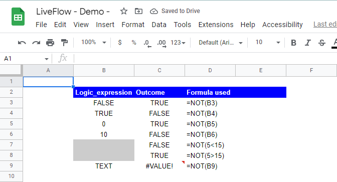
Note: If you input 0 in the formula, it returns “TRUE” as 0 has a logic value of FALSE in Google Sheets, though other numeric values have a logic value of TRUE. You can’t input non-numeric values, such as text. With such input, the NOT function returns “#VALUE!”. (You can refer to non-numeric values as part of logical expressions)

‍

You can see some examples in the following screenshot below.

‍

‍

‍

‍

What formula can you use with the NOT function in Google Sheets?

‍

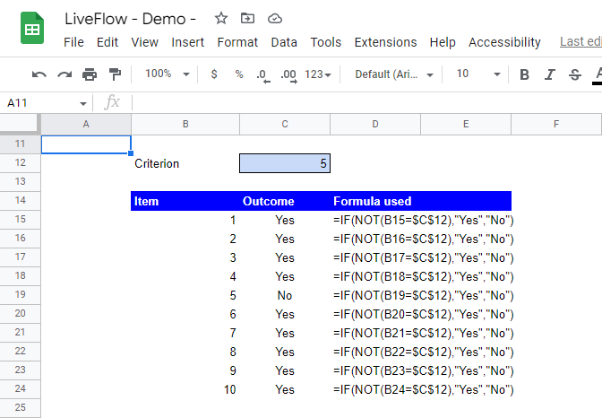
The NOT function is often used in conjunction with other logical functions such as IF, AND, and OR. For example, you can use the NOT function with the IF function to create a formula that performs different actions based on the opposite of a certain condition.

‍

For example, the following formula will return "Yes" if the value in cell B15 (1) is not equal to the value in cell C12 (Criterion: 5), and "No" otherwise:

=IF(NOT(B15=$C$12), "Yes", "No")

‍

You can see other results for other tested values from 2 to 10. As you can see, only when the sampled value is 5 will you get the return value of “Yes”, as described above.

‍

‍

You can also use the NOT function with the AND and OR functions to create more complex logical formulas.

‍