
ISBLANK Function in Google Sheets: Explained
In this article, you will learn how to use the ISBLANK formula in Google Sheets.
What does the ISBLANK formula do in Google Sheets?
The ISBLANK formula is a simple formula that tells you whether a cell is blank and returns “TRUE” when the cell is empty and “FALSE” when the cell has an input. For instance, the formula is helpful in checking if a cell contains hidden characters, overlooked whitespaces, or empty strings (““).
This formula is often combined with the IF function. You can see an example of the combination of the ISBLANK and IF functions in the following section.
How to insert the ISBLANK formula in Google Sheets
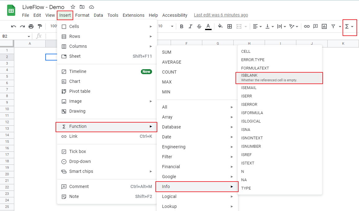
- Type “=ISBLANK” or go to “Insert” → “Function” (or directly navigate to the “Functions” icon) → “Info” → “ISBLANK”.
- Select a cell (not a range) to be checked.
- Press the “Enter” key.
How do I use the ISBLANK formula in Google Sheets?
The general syntax of the ISBLANK function is as follows:
value: This should reference a cell to be checked for its emptiness.
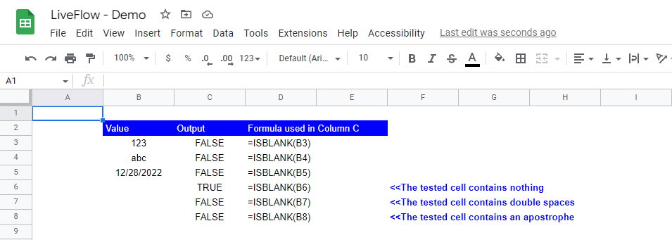
Note: As mentioned above, the ISBLANK formula returns “FALSE” if the cell tested looks blank but contains any value, including whitespaces, the empty string (““), and hidden letters. Consider double-checking and cleaning the cell if you have a “FALSE” result in a cell where you shouldn’t see the FALSE result.
You can see how the function works in the following screenshot. The two examples from the bottom show the cases in which cells look empty but have invisible content.
The following picture shows how the ISBLANK formula can be used in conjunction with the IF and OR functions. This formula processes the information as follows:
(i) If either of Numerator or Denominator is blank, as the OR function returns TRUE, the IF function returns empty strings, which make a cell looks empty, and
(ii) if none of the Numerator or Denominator is blank, as the OR function provides FALSE, the IF formula shows Numerator divided by Denominator.

How do I use the ISBLANK for range in Google Sheets?
To check all cells or one of the cells in a range is empty with the ISBLANK formula, you need to combine it with the other formulas, such as the AND, OR, and ARRAYFORMULA functions. The AND function returns “TRUE”, if all input logic values are “TRUE”.
The OR formula provides “TRUE” when at least one of the logic inputs is “TRUE”. The ARRAYFORMULA allows a function that initially does not accept an array as an argument to take an array as an argument and runs the formula for each cell in the selected array.
If you are interested in learning more about these functions, check out the following articles.
AND Function in Google Sheets: Explained
OR Function in Google Sheets: Explained
ARRAYFORMULA Function in Google Sheets: Explained
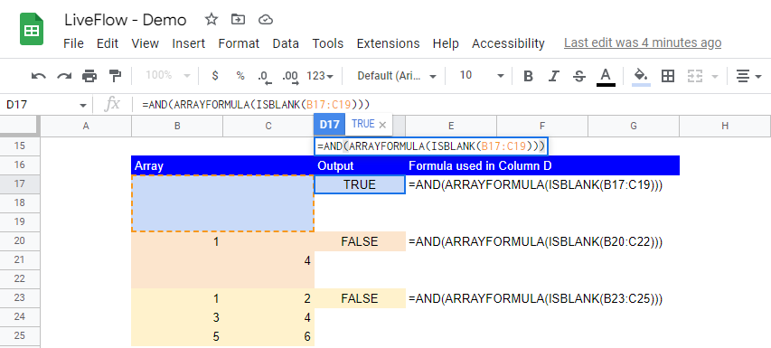
How to check if all cells in a specific range are empty: You can use the AND, ARRAYFORMULA, and ISBLANK function, as shown in the following screenshot. All cells are completely blank in the first 2x3-sized range (highlighted in blue), and the AND formula returns “TRUE”.
In the second (highlighted in orange) or the third (highlighted in yellow) array, as two of the cells or all cells contain values (1 and 4) or (1 to 6), the AND formula gives you “FALSE” for each example.
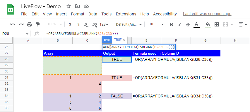
How to check if one of the cells in a specific range is empty: You can combine the OR, ARRAYFORMULA, and ISBLANK functions, as shown in the following screenshot. All cells are completely blank in the first 2x3-sized range (highlighted in green), and the OR formula returns “TRUE”.
In the second array (highlighted in red), as two of the cells contain values (1 and 4), the OR formula still gives you “TURE” because there are four empty cells. However, in the third array (highlighted in purple), as all cells contain values (1 to 6), the OR formula gives you “FALSE” for each example.
How do you make a cell blank if another cell is blank in Google Sheets?
You can combine the ISBLANK formula with the IFERROR function. An example of the mixed formula is as follows: =IF(ISBLANK(A1), IFERROR(0/0,), A1/B1). How does this combined formula work? Assume the IF formula is in cell C1. If a cell checked (A1 in this case) by the ISBLAKN is empty, the IF function returns the value returned by the IFERROR function.
IFERROR(0/0,) always returns nothing (the second argument), which makes a cell blank because 0 divided by 0 is always an error. A point here is to refrain from inputting anything in the second parameter of the IFERROR function.
For example, if you input empty strings (““) as the second argument of the IFERROR formula, the cell looks empty but is not considered blank. You can confirm this by using the ISBLANK formula you learned in this article.


