
How to Use COUNTIFS Function in Google Sheets
In this article, you will learn how to utilize the COUNTIFS formula in Google Sheets.
This formula is beneficial when you want to figure out the number of cells (or values) that satisfy multiple conditions simultaneously.
For example, it is helpful when you need to know the number of items that meet criteria, such as ones sold in a particular lot size by a specific salesperson on a specific date, out of a significantly long sales record.
How to use COUNTIFS formula in Google Sheets
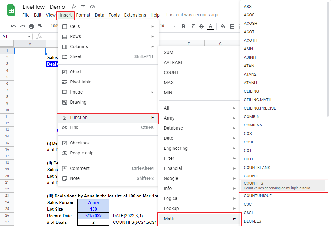
- Type “=COUNTIFS(” or go to “Insert” in the menu bar ➝ “Function” ➝ ”Math” ➝ ”COUNTIFS”
- Select a range for which you apply the first criterion, insert a comma, and input a condition by cell reference or manual input.
- Repeat the second process above until you incorporate all criteria you want to include
- Press the “Enter” key
The generic formula is as follows:
Criterian_range1: This is a set of data to which you want to apply the first criterion.
Criterion1: This is the first standard.
Let’s see a few examples below. Imagine that you are in charge of sales and you need to know the number of deals that meet particular criteria based on a deal list (Sales Record) shown in the picture below.
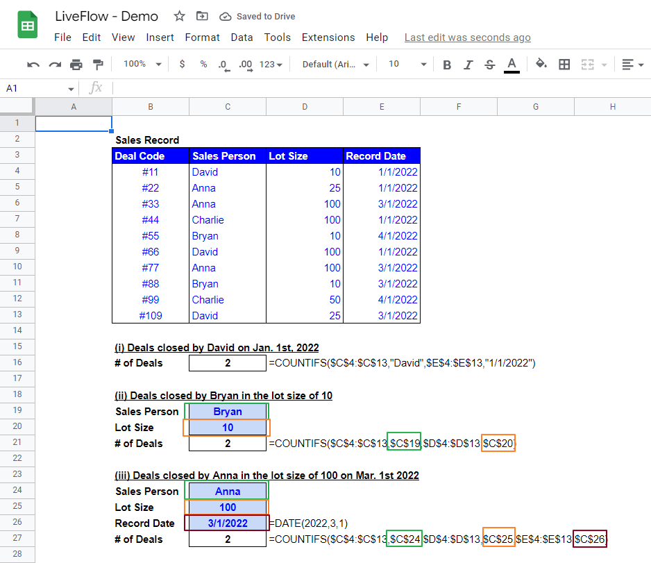
(i) Deals closed by David on Jan. 1st, 2022
In this example, we assume the criteria are Sales Person - “David” and Record Date - “1/1/2022”. As the first condition is a person, the first range should be found in thecolumn C that contains the information about this Sales Person.
The second condition is Record Date, so the second range should be a part of the column E that has the information about the necessary Record Date. In the formula in the screenshot above, both of them are typed manually.
(ii) Deals closed by Bryan in the lot size of 10
The two requirements in this example are Sales Person - “Bryan” and Lot Size - “10”. The first range should be found in the column C again. This time, the column D should be the second filed as the second condition is looking for the Lot Size.
In this sample formula, both conditions are input by cell references rather than manually as you can see in the screenshot. A corresponding pair of cell reference and referred cell is surrounded by the same color boxes. (e.g., Bryan and $C$19 in the formula).
(iii) Deals closed by Anna in the lot size of 100 on Mar. 1st 2022
The last sample formula contains three ranges and criteria, Sales Person - “Anna”, Lot Size - “100”, and Record Date - “3/1/2022”.
All conditions are incorporated with cell references as in the previous example. You can see which part of the formula corresponds to which condition in the picture above.
If you have only one criterion you want to apply to a data set, you can consider using the COUNTIF function. Check this article to learn how to use the COUNTIF formula in Google Sheets.


