
EOMONTH Function in Google Sheets: Explained
In this article, you will learn how to use the EOMONTH function in Google Sheets.
This function is beneficial for checking a month's end date and showing months, such as table headers by month (e.g., monthly financial statement or monthly KPI tracker, etc.).
How to use the EOMONTH formula in Google Sheets
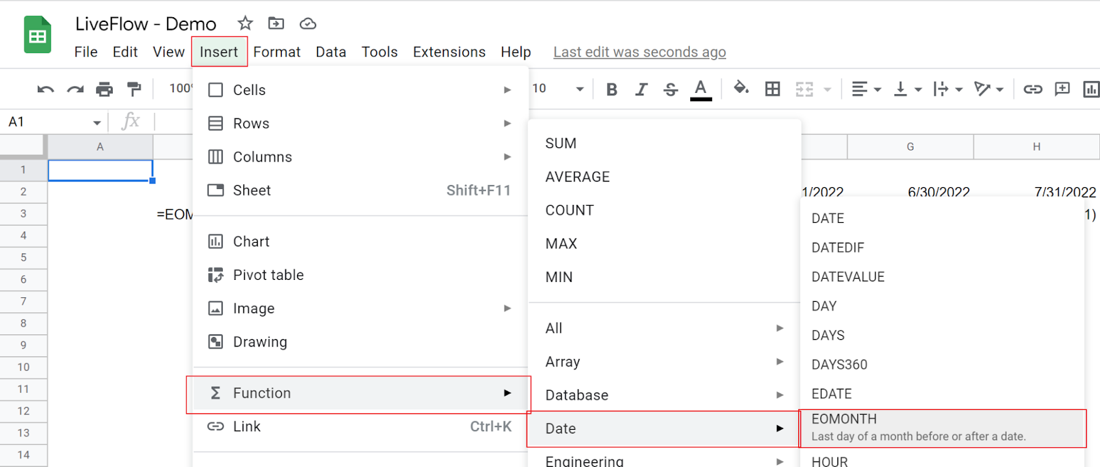
- Type “=EOMONTH(” or go to “Insert” → “Function” → “Date” → “EOMONTH”.
- Input a “start_date” and “months” by manual input or cell reference.
The generic syntax of the function is as follows:
Start_date: This should be a date. This date is a starting point from which the formula calculates the result.
Months: The number of months before (negative figure) or after (positive) the “start_date”. For example, if you enter “3/1/2022” for “start_date” and “2” for this argument, the formula returns the end date of May 2022, as three plus two is five.
As the function shows the end date of a month and adjusts the date shown monthly, it is helpful when you want to know the end date of a month or show months consecutively for a period (e.g., table headers for monthly data).
Assume you are a finance manager and need to create a monthly financial and KPI dashboard for the first half of the fiscal year ending December 31, 2022. You want to make table headers by month. You can use this formula instead of typing all months for your data set.
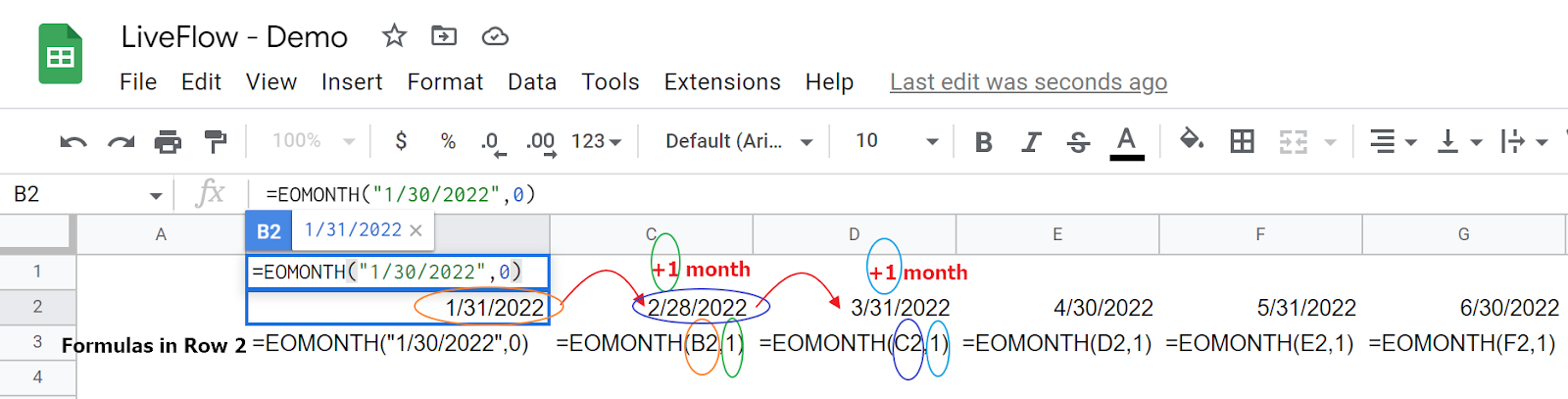
Start_date: For January 2022, we input it manually. Don’t forget to enclose the date with quotation marks. For each month from February to June, we refer to the next cell to the left. (e.g., cell B2(=1/31/2022) in the case of the formula for February (cell C2).)
Months: We input 0 for January because we input a date in January for “start_date” and want to know the end date of January. For each month in the rest of the period, we input “1” because we want to show the end date of a month, which is a month after the previous month.
In this example, we don’t care about the exact date but only the months. So, we are going to change the format of the cells.
- Select a range “B2:G2”.
- Go to the “Format” tab → “Number” → “Custom date and time”.
- In the pop-up window, delete the default input, if any, and click the pull-down menu next to the “Apply” button.
- Choose “Month”, type “-”, reopen the pull-down menu, and choose “Year”.
- Click the “Apply” button.
- Make the texts in the cells bold and white, and color the cells blue.
Steps 3 to 5

After all steps
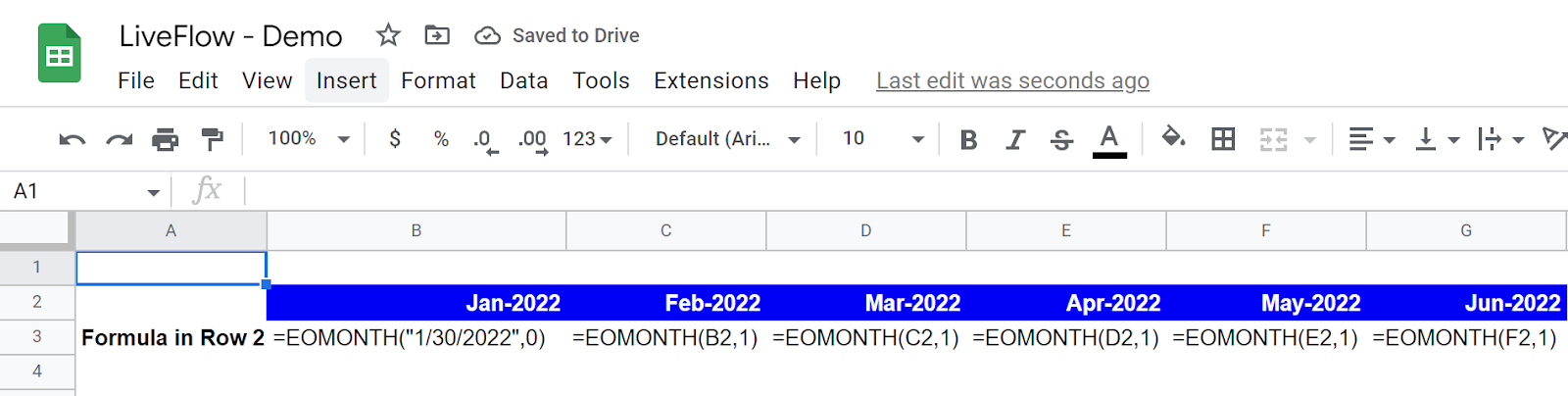
The format change above is just an example. You can customize the formatting of cells and dates according to your company’s coloring order or your preference.
How does HLOOKUP work in Google Sheets?
Read this article to understand how the HLOOKUP function works in Google Sheets.
How do I create a date formula in Google Sheets?
Check this article to learn how to use the DATE formula in Google Sheets: DATE Function in Google Sheets: Explained
How does Google Sheets calculate working days?
You can use the WORKDAYS or NETWORKDAYS functions depending on your purpose.


