How to Use IMPORTRANGE Function in Google Sheets

In this article, you will learn how to refer to a range in another Google Sheets file by the IMPORTRANGE function. In Google Sheets, you can’t refer to another file without any formula, so this function is beneficial for connecting two files and keeping imported information updated.

‍

How to use IMPORTRANGE formula in Google Sheets

1. Type in “IMPORTRANGE” or navigate to the “Insert” tab (or “Functions” icon) → “Function” → “Web” → “IMPORTRANGE”.
2. Open a Google Sheets file you want to refer to.
3. Copy the URL of the file.
4. Insert the URL in the formula and enclose it wilt quotation marks.
5. Type in a sheet name and range in the formula and surround them with quotation marks.
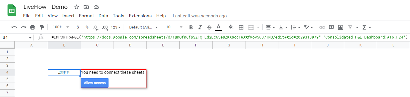
6. As you see “#REF” in the cell and its note stating, “You need to connect these sheets”, click “Allow access” in the note.

‍

The general syntax is as follows:

=IMPORTRANGE(spreadsheet_url, range_string)

Spredseet_url: You need to insert an URL in this argument. The quotation marks must be added at the beginning and end of the URL such as “XXX”.

Range_srting: This argument requires a sheet name and range. The two items must be combined with “!”, an exclamation mark, and enclosed with quotation marks. You can type in Named Range instead of inputting row and column indexes for the range in the referred file. For example, if you want to refer to a range of B2:F17 on a sheet named Sample, the argument should be “Sample!B2:F17”.

‍

Look at a more specific example. Assume you want to refer to the data under the following assumptions.

‍

URL: https://docs.google.com/spreadsheets/d/1BmOfn6fpSZFQ-Ld2Ec65e8ZKX9ccFWggfWov5u37TNQ/edit#gid=2029313979

Sheet: Consolidated P&L Dashboard

Range: A16:F24

‍

With these assumptions, the IMPORTRANGE formula must look as below.

‍

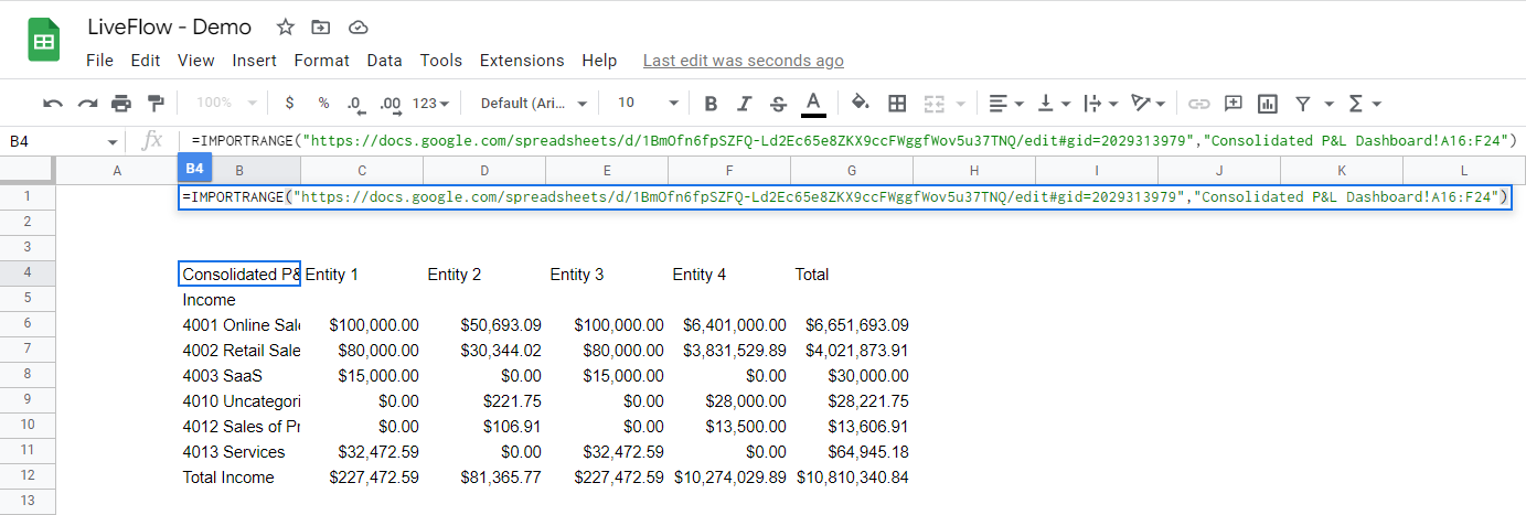
=IMPORTRANGE(“https://docs.google.com/spreadsheets/d/1BmOfn6fpSZFQ-Ld2Ec65e8ZKX9ccFWggfWov5u37TNQ/edit#gid=2029313979”, “Consolidated P&L Dashboard!A16:F24”)

‍

Once you allow access and wait until the formula completes loading, you can see values from the referred range, as shown below.

‍

Note the following points:

1. You need to secure enough space for the formula to spread the imported values.
2. The formula imports values without formatting, row height, or column width. So, you need to copy and paste the formatting in the source file if needed.
3. If there is any update in the selected range in the source file, the IMPORTRANGE function reflects the change immediately, so the imported information is always up-to-date.

‍

What are the other useful functions in Google Sheets?

If you don’t get the solution to your question in this article or you are interested in learning the other useful functions in Google Sheets, you may find the answers in the following articles.

‍

Read the following articles to make some cases for your analysis.

How to Use CHOOSE Function in Google Sheets

How to Use SWITCH Function in Google Sheets

‍

Move on to these articles if you are interested in them.

How to Use RANK Function in Google Sheets - Organize your dataset by ranking items

ARRAYFORMULA Function in Google Sheets: Explained - Use arrays in non-array formulas

SEQUENCE Function in Google Sheets: Explained - Create a grid of sequential numbers

VALUE Function in Google Sheets: Explained - Convert a number, date, and time string to a number

‍

Go to the articles below to learn how to generate random numbers in Google Sheets.

RAND Function in Google Sheets: Explained

RANDBETWEEN Function in Google Sheets: Explained

RANDARRAY Function in Google Sheets: Explained

‍

Navigate to the following posts to learn how to make a hyperlink and import data from another Google Sheets file or a web page.

HYPERLINK Function in Google Sheets: Explained

IMPORTDATA Function in Google Sheets: Explained

IMPORTHTML Function in Google Sheets: Explained

‍

Check the articles below if you want to use translation-related functions in Google Sheets.

GOOGLETRANSLATE Function in Google Sheets: Explained - Translate one language to another.

DETECTLANGUAGE Function in Google Sheets: Explained - Identify the language used in a specified cell.

‍

Analyze your live financial data in a snap

Are you learning this formula to visualize financial data, build a financial model, or conduct financial analysis? In that case, LiveFlow may help you automate manual workflows and update numbers in real-time. You can access various financial templates on our website, from the simple Income Statement to Multi-Currency Consolidated Financial Statement. You can also customize these templates as you want without breaking the automated data inflow.

To learn more about LiveFlow, book a demo.