FILTER Function in Google Sheets: Explained

In this article, you will learn how to use the Filter function in Google Sheets. The formula is helpful when you need to pull out specific information under condition(s).

‍

How to use the Filter formula in Google Sheets

1. Type “=FILTER(” or navigate to the “Insert” tab (or “Functions” icon) → “Function” → “Filter” → “FILTER”.
2. Select the source data in “range”.
3. Input as many conditions as you have.
4. Press the “Enter” key.

‍

The general syntax is as follows:

=FILTER(range, condition1, [condition2, …])

Range: This is the source data to which the FILTER function applies conditions. The FILTER function projects only information that meets the requirements defined.

Condition1: The first condition data must meet to be shown by the FILTER formula.

Condition2(Optional): You can include more than one standard if needed.

‍

Note: all conditions should be the same type (row or column). Using both row and column conditions is not allowed. Also, condition arguments should have precisely the same length as “range”. Lastly, do not forget secure enough space for the data pulled out.

‍

The FILTER function is helpful when you need to pull out or focus on specific data or information that meets the criteria.

‍

Assume you have a profit list that contains the project name, project leader, budget, and deadline. You want to pull out the data on the projects that meets specific criteria. Before doing that, see the following example showing how to excerpt a part of the original data set. Imagine you are going to check each budget amount equal to or more than $5,000.

‍

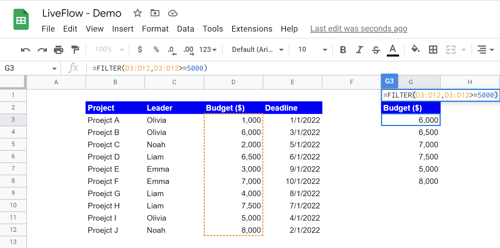
In this example, the formula in cell G3 contains the following arguments.

Range: D3:D12

Condition1: D3:D12>=5000

As you can see, you can select the same range for both “range” and “condition”. Note you don’t need to enclose these marks, “>” and “=”, with quotation marks in this formula. Don’t forget to prepare a table header and enough space for the formula to spread pulled values.

‍

If you want to search the data set for projects whose leader is “Olivia”, you can enter the “=FILTER(C3:C12, C3:C12=”Olivia”)”. If you need to sort the projects whose deadline is on or earlier than “7/1/2022”, you can use the formula like “=FILTER(E3:E12, E3:E12<=date(2022,7,1)”.

‍

How do I filter data in Google Sheets with multiple criteria?

The following example shows how the function works with multiple conditions. Assume you want to see projects that meet the following requirements.

1. The project leader is “Olivia”.
2. The budget amount is equal to or more than $5,000.
3. Deadline is on or after 3/1/2022.

‍

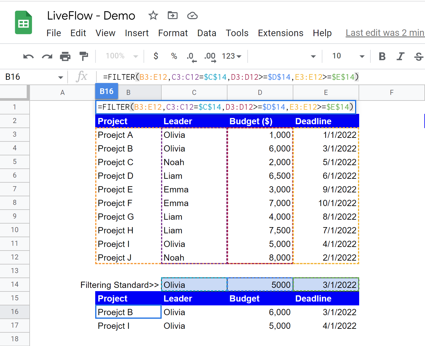
In this example, the formula in cell B16 contains the following arguments.

Range: B3:E12

Condition1: C3:C12>=$C$14

Condition2: D3:D12>=$D$14

Condition3: E3:E12>=$E$14

The formula returns values in the same number of columns in the case of conditions by column (this example) and in the same number of rows when requirements are based on row values. You can enter requirements by cell reference as well as shown above.