
Conditional Formatting Based on Another Cell Value in Google Sheets: Explained
In this article, you will learn how to apply Conditional Formatting to cells based on another cell value in Google Sheets. If you want to understand the basic Conditional Formatting rules, check this article.
How to use Conditional Formatting based on another cell
- Navigate to the “Format” tab and select “Conditional formatting”.
- A pop-up menu for Conditnoa Formatting shows up on the right side.
- Select the “Single color” tab in the menu.
- Choose “Custom formula is…”
- Enter a formula you want to apply to a selected field.
- Define the cell and font style in which a cell value meets the formula.
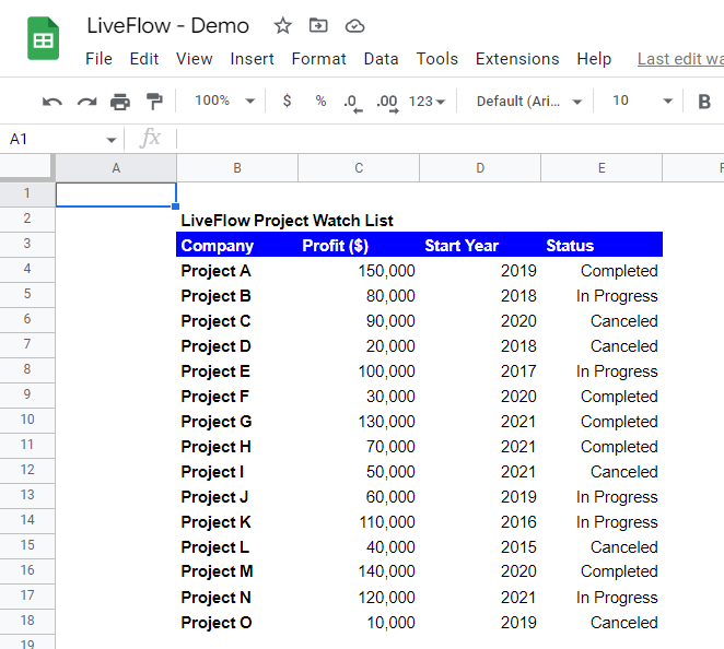
Let’s see an example. Imagine you are a corporate planning manager and have your company’s project list. You want to check which project is generating profit equal to or over a certain amount and add those projects to a watch list as critical projects.
However, you want to make the standard changeable because you have no idea how many projects meet a specific criterion. The imaginary data set is as follows.
To implement the standard, you need to:
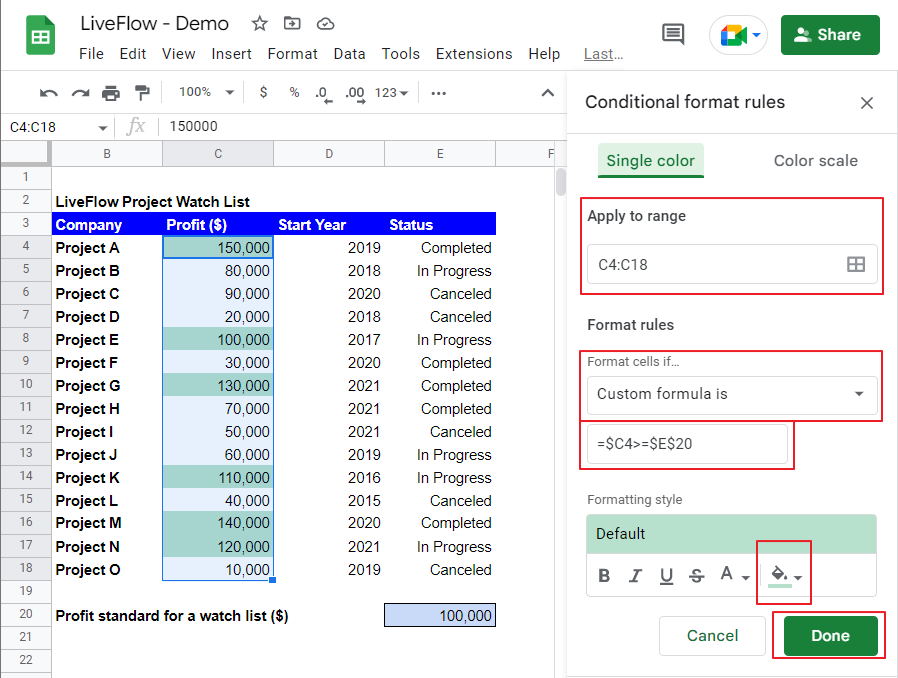
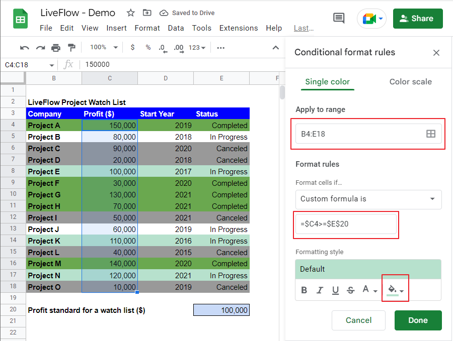
- Set the target range as C4:C18.
- Choose “Custom formula is…”.
- Enter the following formula in a text box “=$C4>=$E$20”.
- Click “Done” at the bottom right.
The key points you should bear in mind are;
(i) if the range selection is correct as the coloring and style rule is applied to the selected range entirely;
(ii) if the signs used in the formula are correct; and
(iii) whether the formula is valid and is input correctly. The formula needs to start with the “=” sign. You must check if the reference type, whether relevant, partial absolute, or absolute, is appropriate.
In the example, you want to test each cell (from C4 to C18) in Column C, so you need to lock the column of the tested cells by adding “$” next to the “C” in the formula.
For the standard in cell E20, as it is always there wherever the tested cell is, you make it an absolute reference by adding “$” next to both the column and row indexes like “$E$20”.
If you want to change the standard from $100,000 to another value, type the value directly in cell E20. Then, the color of cells changes accordingly.
After understanding the number of projects with a profit equal to or over $100,000, you realize that some projects are already completed or canceled. So, you want to highlight them in different colors. You also need to color the entire row for items completed or canceled. So, you decide to take the following approach.
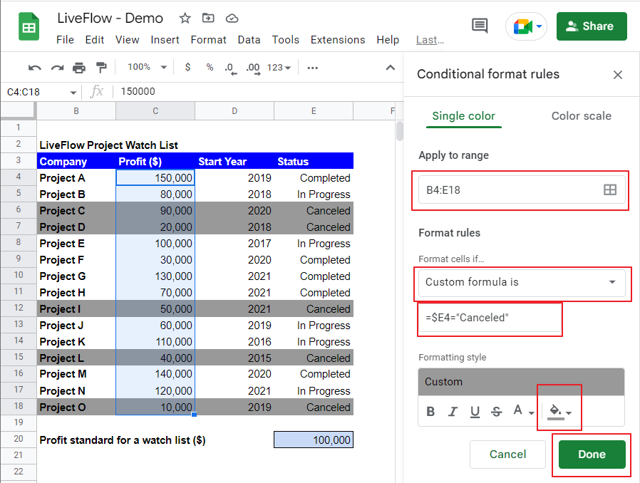
- Grey out projects that have “Canceled” status.
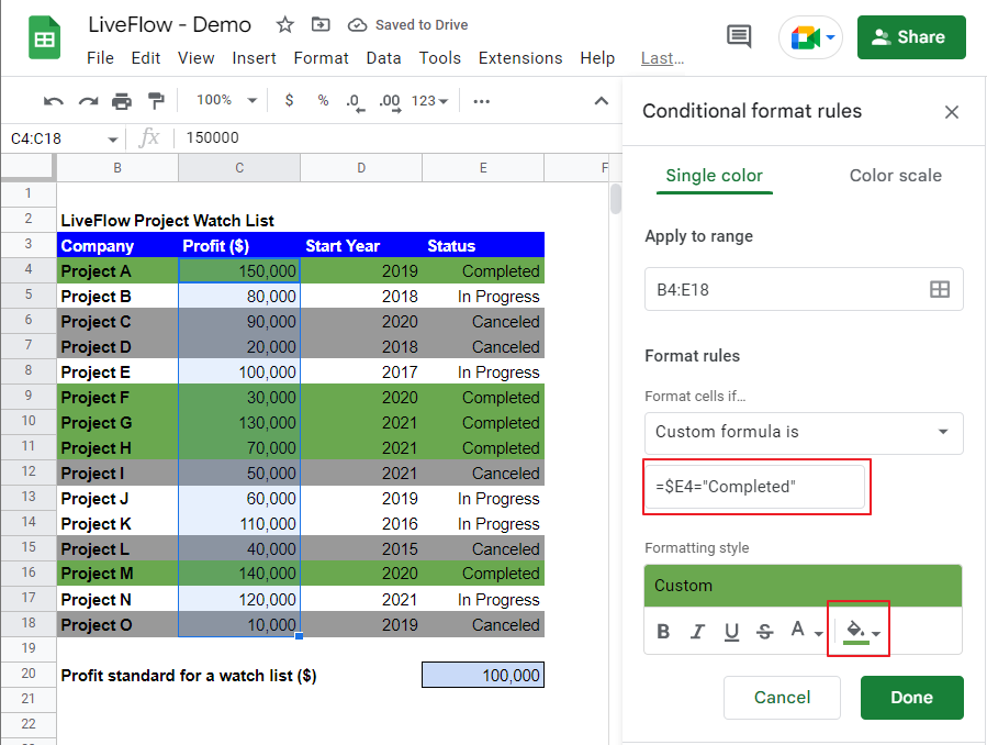
- Highlight projects in dark green that has “Completed” status.
- Highlight projects with profit over or equal to $100,000 in light green.
The first rule
The range should be the entire table. You want to run a test for Column E in this rule. So, a tested cell should be a partial absolute reference such as $E4 again in the custom formula.
The entire formula should be “=$E4=”Canceled”” because you want to check if the status of a project is “Canceled” or not. Finally, change the fill color to dark grey.
The second rule
The second rule is the same as the first rule except for the custom formula and the fill color. This time, the formula should be “=$E4=”Completed”” to check if a selected cell is “Completed” or not.
The third rule
The third rule looks almost similar to the principle you created for Column C in the first example. However, as you want to color a row instead of a cell containing a tested value, the range should cover the entire list, as the first and second rules do.
As a result of the processes, you get the list highlighted as above. The projects you need to add to a watch list are Projects E, K, and N.
How do the Conditional Formatting rules work with each other if there is a conflict?
Note that the rules are prioritized in ascending order - the first rule in the Conditional Formatting list is most prioritized. In the approach above, the rules’ priority is 1>2>3. If you want to change the order of the rules, you can do it in the list by drugging and releasing a rule, as shown below.