
How to Use MODE Function in Google Sheets
In this article, you will learn how to use the MODE formula in Google Sheets.
The mode number (in math) means the most frequent figures in a data set.
For example, if you have a set of numbers such as {1, 2, 3, 3, 4, 4, 4, 5, 5}, the mode is 4 as it appears three times in the data set, and others do equal to or less than two times. The MODE function helps you find the mode in a series of numbers.
How to use the MODE formula in Google Sheets
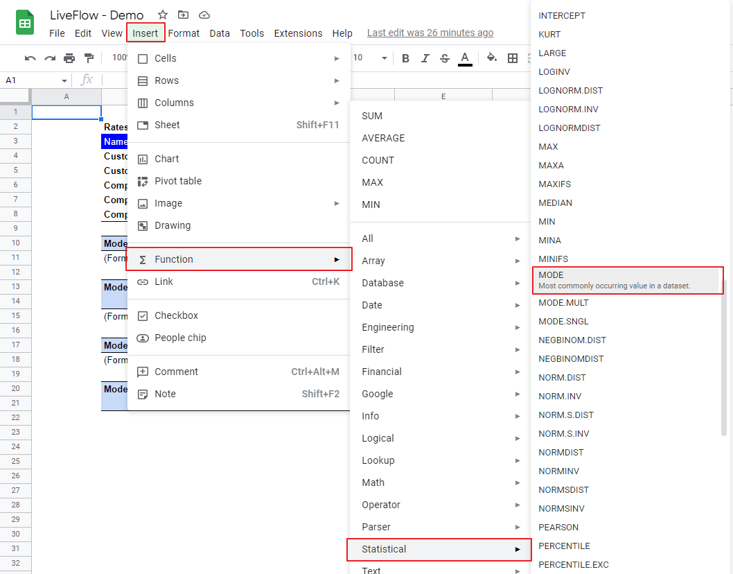
- Type “=MODE(” or go to “Insert” → ”Function” → ”Statistical” → ”MODE”.
- Select a set of data from which you want to find the mode. If you want to incorporate non-adjacent areas, you can include them by punctuating them with a comma(s).
- Press the “Enter” key.
The generic formula is as follows:
Value 1: A set of data based on which you want to figure out the mode number.
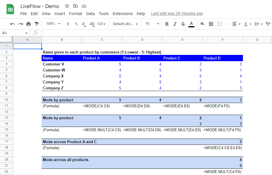
Let’s see some examples. Imagine you review five customer rates given to four types of products:
(i) Mode by product
This is simple. You can just select a part of the column for each product. For example, the MODE formula in cell C10 (for Product A) contains a range of C4:C8, specifically 5, 4, 5, 4, and 5, and you get 5.
However, see a column for Product C containing 2, 3, 5, 3, and 2. There are two 2s and two 3s, so the answer should be 2 and 3 for this part of the column. Here is a weak point of the MODE function.
A set of data likely contains more than one of the most frequent figures, but the MODE function can return only one of them. If you don’t know the most frequent number in a data set, you should use MODE.MULT formula instead. (You can type “=MODE.MULT” or find the formula just beneath the MODE function in the formula list).
You can use this function as the MODE function in data input. This function returns all mode figures in a data series (if any). Look at the second “Mode by product” section. You can see all mode numbers show up.
Remember to secure enough cells for the number of anticipated values. You can insert rows and columns later so the formula can show all answers.
(ii) Mode across Product A and C
This example might be a little tricky. As mentioned above, if you want to select non-adjacent fields as a data set, you can use a comma(s). Select a part of the column for Product A (C4:C8), add a comma, and select a part of the column for Product C (E4:E8).
The group of numbers contains {5, 4, 5, 4, 5, 2, 3, 5, 3, 2}, and thus, the most frequent number is 5. Therefore, the mode is 5.
(iii) Mode across all products
As you can see in the screenshot, you can select a table as a set of data which include twenty figures for all product.
In this case, we don’t know how many of the most frequent numbers there are in the data set, so let’s use MODE.MULT formula instead of MODE function.
How do you find the mean and median in Google Sheets?
If you are interested in finding the mean and median in a set of numbers in Google Sheets, you can use the AVERAGE and MEDIAN functions. Check the following pasges for the AVERAGE and MEDIAN formulas.
How to Use MEDIAN Function in Google Sheets
How to Use AVERAGE Formula in Google Sheets